Open Journal of Fluid Dynamics
Vol.3 No.2(2013), Article ID:33652,7 pages DOI:10.4236/ojfd.2013.32014
Numerical Simulation of Water Impact on a Wave Energy Converter in Free Fall Motion
School of Computing, Mathematics and Digital Technology, The Manchester Metropolitan University, Manchester, England
Email: L.Qian@mmu.ac.uk
Copyright © 2013 Zheng Zheng Hu et al. This is an open access article distributed under the Creative Commons Attribution License, which permits unrestricted use, distribution, and reproduction in any medium, provided the original work is properly cited.
Received March 4, 2013; revised April 5, 2013; accepted April 15, 2013
Keywords: Wave Energy Converter; Manchester Bobber; Cartesian Cut Cell; Free Surface Capturing and Artificial Compressibility Method
ABSTRACT
Results are presented for the 3D numerical simulation of the water impact of a wave energy converter in free fall and subsequent heave motion. The solver, AMAZON-3D, employs a Riemann-based finite volume method on a Cartesian cut cell mesh. The computational domain includes both air and water regions with the air/water boundary captured automatically as a discontinuity in the density field thereby admitting break up and recombination of the free surface. Temporal discretisation uses the artificial compressibility method and a dual time stepping strategy. Cartesian cut cells are used to provide a boundary-fitted grid at all times. The code is validated by experimental data including the free fall of a cone and free decay of a single Manchester Bobber component.
1. Introduction
A popular class of wave energy converter (WEC) consists of floating bodies which oscillate with one or more degrees of freedom and whose horizontal dimensions are small in comparison to the wave length. Such bodies are point absorbers and they essentially convert their heave motion into useful energy. Several such WECs composed of one or more point absorbers are currently under development. Examples include the Manchester Bobber [1] details of which will be given later, the  [2] and Wavestar [3]. At present, intensive research is being carried out on shape optimization of the point absorbers from the point of view of power absorption (see Alves et al. [4] and Vantorre et al. [5]) but the issue of their survivability has not been fully addressed. These point absorbers may be subject to high wave loading during storms and in fact may be subject to slamming as they are tossed around by large waves. Hence, there is a great need for simulation tools that can predict the wave impact loads on these point absorbers.
In this paper, attention is focused on a particular WEC: the Manchester Bobber henceforth referred to as “the Bobber”. The Bobber was designed by researchers at the University of Manchester in the UK and consists of an array of novel heaving point absorbers which generate oscillatory shaft motion that is converted to unidirectional rotation through a freewheel/clutch system which in turn drives an electricity generator. In order to assess the survivability of the Bobber, a full set of flow variables is required e.g. pressure and velocity field, as well as integrated effects like forces and device response as outputs from laboratory experiments or CFD predictions. In this paper, the numerical study is focused on an isolated Bobber under water impacts but the same code could be used to simulate violent wave impacts.
Research work on the water impact problem has been mainly for 2D cases. Greenhow and Lin [6], Greenhow [7], Zhao and Faltinsen [8] and Mei et al. [9] studied the hydrodynamics of water entry of rigid bodies both theoretically and experimentally. All these studies were for bodies entering the water at constant speeds which are unrealistic. In the real world bodies undergo acceleration and deceleration as they enter water so this should be considered. In free fall motion, the numerical results for a wedge entering water were compared with the experimental and theoretical work of Campbell and Weynberg [10] and Wu et al. [11]. More recently, experimental investigation of the pressure distribution on a free falling wedge entering water was conducted by Yettou et al. [12]. In addition, Backer et al. [13] investigated both prescribed motion and free fall motion for a cone in 3D. Our previous work (Hu et al. [14]) on related water impact problems has involved the prescribed motion of 3D rigid solid bodies. In this study, we extend our work to water impact problems of free fall motion for a cone, a hemisphere and the Bobber.
Our in-house AMAZON-3D finite volume code solves the incompressible Navier-Stokes equations in both air and water regions and treats the free surface as a contact surface in the density field that is captured automatically in a manner analogous to shock capturing in compressible flow. Meshing uses the Cartesian cut cell method which automatically produces a body fitted mesh for static or moving solid bodies. Solid objects are cut out of a background Cartesian mesh leaving a set of irregularly shaped cells whose surfaces coincide with the boundary of the solid. There is no requirement to re-mesh globally for the case of a moving body. All that is required is to update the cut cell data at the body surface for as long as the body motion continues. The background mesh needs not be uniform and in fact non-uniform Cartesisn meshes were used in our simulations with small cells around the body for improved resolution. We have used the code to study wave loading on a Bobber-type WEC device under extreme wave conditions in a numerical wave tank (Hu et al. [15]).
This paper focuses on the numerical modelling of the vertical slamming on a floating Bobber and the associated pressures that might be expected when slamming occurs. The code has been validated by the free fall of a cone and free decay of a Bobber. Results including the vertical displacement will be presented for the water impact of bodies in free fall motion.
2. Numerical Method
2.1. 3D Cartesian Cut Cell Mesh
An essential component of a CFD simulation is the mesh generation and it is particularly important for the present case because of the movement of the solid body within computational domain.
It is well known that the finite volume method (FVM) involves discretization of the flow domain of interest and then integration of the flow equations over elemental cell volumes. The method enables correct flux balances across cell boundaries and conserves momentum throughout the grid. Therefore, advantage may be gained by using the FVM since the dependent variables remain at all times referenced to a Cartesian frame even when boundary-fitted using cut cells. The remainder (majority) of the cells are uncut flow cells that be treated in a straight forward manner. However, whilst the Cartesian cut cell algorithms can easily accommodate moving boundaries, there are pathological cases where the approach can sometimes provide relatively poor resolution of some particular geometric features. For example, a numerical instability may occur locally within the flow solver if cut cells become arbitrarily small. To overcome this problem, cell merging is implemented as in Clarke et al. [16], Yang et al. [17] and Qian et al. [18] who successfully applied the technique in many applications within aerospace and hydrodynamics. The basic idea is to combine the small cut cell with its neighbouring cells to form a new cell with the interface between merged cells ignored. A minimum volume criterion Vmin is specified for the cut cell volumes before the flow simulation starts. If the volume of a cut cell is less than Vmin that cell will be merged with neighbouring cells in the direction of the shortest side face otherwise the cut cell will remain unchanged. For computational efficiency cut cell algorithms generally assume a maximum number of cuts within a cut cell which may result in some sub-grid scale geometric features of the body being approximated and this approximation may in principle vary slightly from one time step to another if the body is in motion. However, we find that such higher-order approximations are generally consistent with the accuracy of the associated body’s surface description.
2.2. Governing Equations
The integral form of the Euler equations for 3D incompressible flow with variable density can be written as
 (1)
(1)
where Q is the vector of conserved variables which encloses the time dependent domain of interest V, F is the flux vector function and n is the outward unit vector normal to the boundary S. B is a source term for body forces. Q, F and B are given by
 (2)
(2)
 (3)
(3)
 (4)
(4)
where
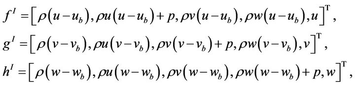
and u, v and w are the flow velocity components and ub, vb and wb are the velocity components of the boundary S which are zero when the boundary is stationary. ρ is the density, p is the pressure, β is the coefficient of artificial compressibility and g is the gravitational acceleration.
2.3. Numerical Solution
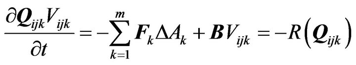
We can then discretize Equation (1) over each cell within the flow domain using a finite volume formulation, this gives
 (5)
(5)
where  is the average value of Q in cell
  stored at the cell centre and
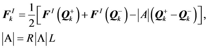
  denotes the volume of the cell. Fk is the numerical flux across the face k of the cell, ΔAk is the area of the face and m is the number of faces of the cell. The convective flux Fk is evaluated using Roe’s approximate Riemann solver, which assumes a 1D Riemann problem in the direction normal to the cell face and has the form
 (6)
(6)
where  and
and  are the reconstructed values on the right and left at face k and A is the flux Jacobian evaluated by Roe’s average state. The quantities R, L and
  are the right and left eigenvectors of A and the eigenvalues of A respectively.
To achieve a time-accurate solution at each time step of the unsteady flow problem a first-order Euler implicit difference scheme is used to discretise Equation (5) as
 (7)
(7)
Introducing a pseudo-time derivative into Equation (7), this gives
 (8)
(8)
where τ is the pseudo-time and . The right-hand side of Equation (8) can be linearized using Newton’s method at the m+1 pseudo-time level and then can be written in the matrix form
 (9)
(9)
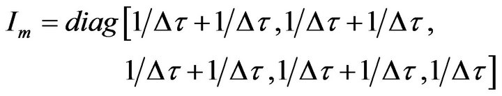
where
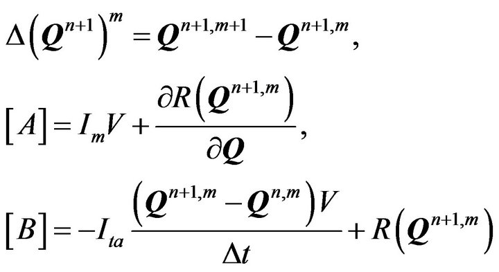
and Im should be defined as
 .
.
When  is iterated to zero, the density and momentum equations are satisfied, and the divergence of the velocity at time level n + 1 is zero. The system of equations can be written in matrix form as
 (10)
(10)
where D is a block diagonal matrix, L is a block lower triangular matrix and U is a block upper triangular matrix. Each of the elements in D, L and U is a  matrix. An approximate LU factorization (ALU) scheme as proposed by Pan and Lomax [19] can be adopted to obtain the inverse of equation (10) in the form
 (11)
(11)
Within each time step of the implicit integration the sub-iteration is terminated when the L2 norm of the iterates process
 (12)
(12)
is less than a specified limit ε and  in this paper.
2.4. Boundary Conditions; Free Surface and Force Calculations
For all test cases non-reflecting boundary conditions are applied at the top boundary allowing air to leave or enter the domain freely. The remaining boundaries are set as rigid walls.
At the interface between two immiscible fluids, the present method assumes that the system of equations for non-homogeneous, incompressible flow can treat the free surface numerically as a contact discontinuity in the density field. Special procedures to track the free surface are thus unnecessary since the free surface is captured automatically. It is asserted that the numerical solution of Equation (1) for a system containing one or more free surfaces will converge to the correct unique solution.
In the current approach, the pressure value p can be calculated from the term p/β in Equation (2) by multiplying by β. The total force is then obtained by integrating the pressure field along the body surface
 , where Sb is the area of the body surface as defined by the cut cell surface fitting.
3. Results
To simulate water impact on floating body, the body must be allowed to move freely according to the interaction between the fluid and the body. In this paper, our numerical simulation with body motion is used to heave only, which is main part of the body motion in this problem. In the following calculations, the density ratio of water to air is taken as 1000:1. The location of the free surface, i.e. the air/water interface, is defined as the density contour with the value 500 kg∙m−3. The value of the gravitational acceleration is taken as 9.8 ms−2. The typical physical time step used is  and the pseudo time step is set as
 . The value of the artificial compressibility parameter is
 .
.
3.1. Free Fall of a Cone with Deadrise Angle 20˚
The first test involves a free falling of a cone with deadrise angle 20˚ into still water. The physical tank tests are described by Backer et al. [13]. They tested a model along tightened steel wires to make sure that the floater fell down without experiencing small rotations and big horizontal motion, They used a water tank with dimensions (l × w × h) of 1.2 m × 1.0 m × 1.25 m and our numerical domain has the same size except for height which is set to 2.6m as the body was positioned 1.0 m above the still water surface prior to release. Two nonuniform meshes were used: One is used for a mesh spacing in the refined regions close to the body geometry of 0.020 m with a total of 42 × 38 × 114 = 181,944 cells, the other is used for a mesh spacing in the refined regions close to the body geometry of 0.016 m with a total of 56 × 50 × 142 = 397,600 cells. The maximum radius of the cone is 0.15m with the height of the top cylinder section set to 0.08 m (see Figure 1) and the mass of the cone is m = 4.1 kg.
In the physical experiments, the time history of pressure on the cone surface was recorded during the impact at two locations (S1 and S2) with a horizontal distance of 0.04 m and 0.09 m respectively from the symmetrical axis as shown in Figure 2. To compare with the experimental data, the real time starting from the moment that cone is released from 1 m above the water surface has been used. In Figure 3 the calculated pressures at S1 and S2 on two meshes are compared with those from the physical experiments showing good agreement in terms of the typical shape of impact pressure, which consists of a steep rise of pressure followed by a gradually decreas-
Figure 1. Cone with deadrise angle of 20˚.
Figure 2. Position of the pressure sensors S1 and S2.

Figure 3. Comparison of pressure history at positions S1 and S2.
ing part on the right side of the peak. However, there is a substantial difference in the peak pressure values between the experimental and numerical data. For example, the values of the peak pressure are 0.455 bar for the finer mesh and 0.404 bar for the coarser mesh but for the experimental this value is 0.719 bar. This indicates further mesh refinements especially for the region near the surface of the cone are still needed. To show this and to save the computation time, an axi-symmetric version of the free surface code has been applied to simulate the same flow problem. Three levels of grid (dx = dy = 0.005, 0.0025 and 0.00125 m respectively) have been used with a time step of 
![]() . In Figure 4, the calculated surface pressure value at S2 is compared with the experimental ones, from which it can be seen that to get the peak pressure values very fine mesh must be used. The calculation is repeated for the intermediate mesh spacing of dx = dy = 0.0025 m using four different time steps and the results are shown in Figure 5.
. In Figure 4, the calculated surface pressure value at S2 is compared with the experimental ones, from which it can be seen that to get the peak pressure values very fine mesh must be used. The calculation is repeated for the intermediate mesh spacing of dx = dy = 0.0025 m using four different time steps and the results are shown in Figure 5.
From these results, it can be concluded that for the test case of a free falling cone impacting on water surface the occurrence of peak surface pressures is an extremely localised phenomenon in both space and time, so ex-
Figure 4. Grid refinement tests using the axi-symmetric code for the surface pressure at position S2.
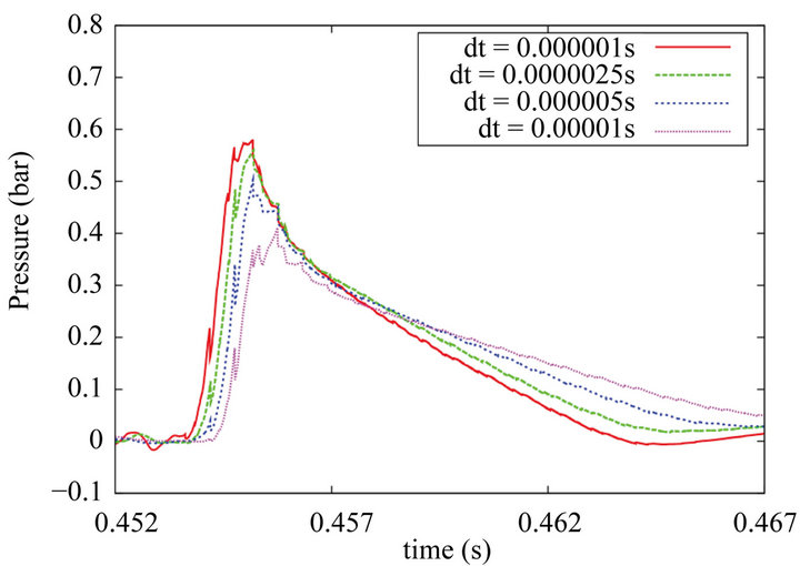
Figure 5. Effect of time step on the peak pressure values at position S1 using the axi-symmetric code.
tremely small mesh size and time step at least locally must be used in order to capture those moments accurately. This highlights the need for both spatially and temporally adaptive solutions for such flow problems. On the other hand, the integrated global values such as the impact force, body acceleration and moving speed are much less affected by the localised extreme pressure values. For the same interval time as above, Figure 6 shows the vertical velocity (absolute value) from the two meshes compared with those from the physical experiments. During the impact, the velocity of the cone, according to the experimental data, has dropped from 4.4 m/s to 2.6 m/s, while for the numerical result on the fine mesh the corresponding change is from 4.4 m/s to 2.4 m/s. Similarly, for the acceleration both results are also in reasonable agreement with each other.
The small differences in velocity may be due to the laboratory model not being constrained to heave motion only. Other reasons which explain the differences may be due to the volume of cone (or associated buoyancy force) being slightly different from the laboratory model owing to small inaccuracies in the surface fitting of the geome-
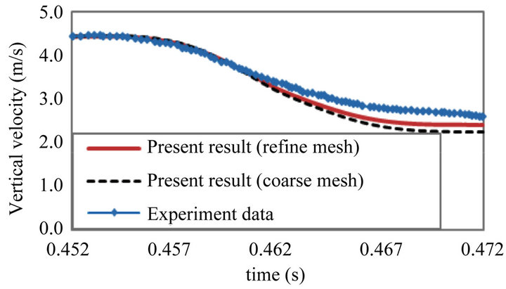
Figure 6. Comparison between experimental data (Backer et al. (2008) and numerical results for the vertical velocity.
try used in the cut cell model (see Figure 1).
The simulations were carried out using one processor of a 600 MHz NEC vector computer with the CPU times of 2 days for the coarse mesh and about 5 days for the finer mesh.
3.2. Free-Decay Test for a Manchester Bobber
This test case simulates the free-decay of the Bobber as described in the physical tank tests by Thomas et al. [20]. In the physical experiments, the oscillating motion of the Bobber is controlled by the weight of the Bobber and a counterweight, which is connected through a pulley system to the Bobber as shown in Figure 7. In the numerical simulation the formula for the movement of the system is given by
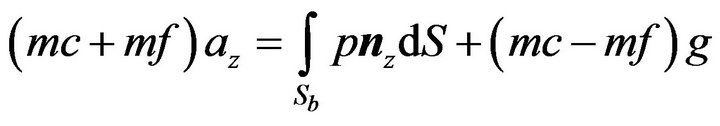 (13)
(13)
where the total mass equals the Bobber mass of mf plus the counterweight mass mc,  is the acceleration in the vertical direction positive upward and the integration on the right-hand side calculates the dynamic force from the pressure on the wetted area of the Bobber in the vertical direction only. According to the experimental tests by Thomas et al. [20], the Bobber mass mf = 2.1 kg and the counterweight mass mc = 1.0 kg will be used in the test. In our numerical tank, the Bobber is allowed to move in vertical motion only dictated by its body weight and the total forces.
3.2.1. The Drop Test
In this test, the geometry of the Bobber is illustrated in Figure 7. The geometry of the Bobber is a flat-bottomed cylinder of radius 0.074 m with a corner radius of 0.033 m. The vertical sides extend to 0.085 m above the flat base and a conical upper surface with a 30 degree base angle decreases the radius of the geometry to 0.025 m at the upper cylindrical section. Figure 8 shows the initial position of the flat-base Bobber at about 0.001 m above the still water surface prior to release. The outer dimensions of the computational domain are 2.0 m × 2.0 m ×
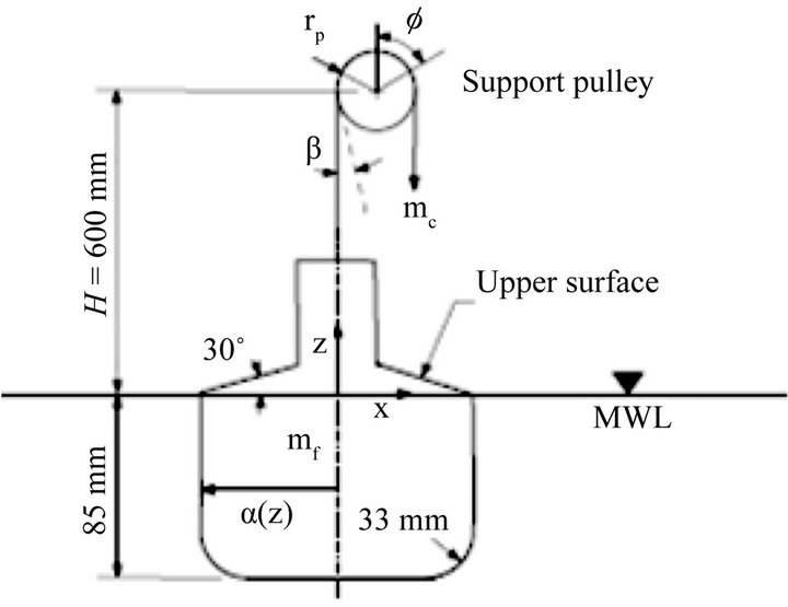
Figure 7. Schematics for the experimental set-up.
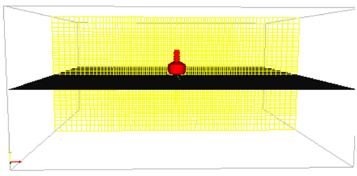
Figure 8. The initial position for the drop test.
1.0 m with a water depth of 0.5 m. A non-uniform mesh is used with 88 × 88 × 48 = 371,712 cells with a mesh spacing of 0.016 m in the refined regions close to the body geometry. Figure 9 shows the equilibrium position of the Bobber at t = 9.0 s, where the Bobber’s base is 0.08 m below the still water surface. Figure 10 shows a comparison of the time history of the vertical displacement obtained in the numerical tank and the experimental observations. The results are in reasonable agreement in terms of both amplitude and decay rate.
3.2.2. The Rise Test
In this test, the initial position of the Bobber in terms of its base is set at 0.16 m below the still water surface (see Figure 11). All other parameters are the same as in the drop tests. Figure 12 shows the final equilibrium position of the Bobber after 9.0 s of simulation, where the penetration depth of Bobber is 0.08 m, which is the same as in the drop test. The results (see Figure 13) again show a reasonable agreement with the measurement for the vertical displacement of the Bobber.
4. Conclusion
In this paper, the motions of solid rigid bodies entering water through free fall moving in heave motion were simulated numerically. A number of tests were performed including the water entry of a rigid cone and a generic heave-type wave energy device called the Man-
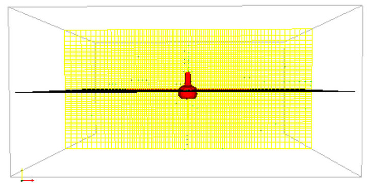
Figure 9. The final equilibrium position for the drop test.
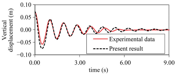
Figure 10. Comparison between experimental data (Thomas (2008)) and numerical results for the vertical displacement.
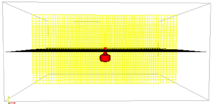
Figure 11. Initial Bobber position for the rise test.

Figure 12. Final equilibrium bobber position for the rise test.
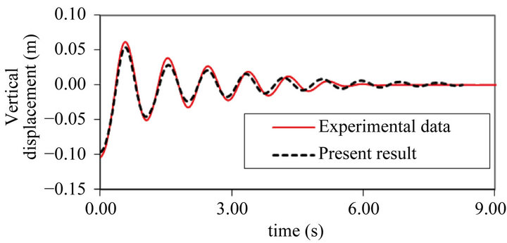
Figure 13. Comparison between experimental (Thomas (2008)) and numerical results for vertical displacement.
chester Bobber. Additionally, free decay tests for the Bobber were carried out. Where available, the numerical results were compared to those from laboratory experiments, which show the potential of the present simulation method for dealing with 3D water/body interaction problems. In particular, the code is able to handle moving solid bodies of arbitrary complexity via the Cartesian cut cell approach and also to deal with complex free surfaces by capturing them automatically as contact discontinuities in the density field. The code has shown the capability for simulating heaving wave energy converters and is able to predict impact forces from slamming which will be useful for survivability assessment studies. Although not demonstrated here, the code is also able to deal with general wave/body interactions and so, given sufficient compute power, would be able to model the performance of generic wave energy converters.
5. Acknowledgements
This work was supported by the UK Engineering and Physical Sciences Research Council (EPSRC) under grant reference EP/D077621 for which the authors are most grateful. The authors would also like to thank T. Stallard, S. Weller and S. Thomas (Manchester University), for their experimental data for the free decay tests of the Manchester Bobber.
REFERENCES
- http://www.manchesterbobber.com
- http://www.seewec.org
- http://www.wavestarenergy.com
- M. Alves, H. Traylor and A. Sarmento, “Hydrodynamic Optimization of Wave Energy Converter Using a Heave Motion Buoy,” The 7th European Wave and Tidal Energy Conference, Portugal, 2007.
- M. Vantorre, M. Banasiak and R. Verhoeven, “Modelling of Hydraulic Performance and Wave Energy Extraction by a Point Absorber in Heave,” Applied Ocean Research, Vol. 26, No. 1-2, 2004, pp. 61-72. doi:10.1016/j.apor.2004.08.002
- M. Greenhow and W. M. Lin, “Non Linear Free Surface Effects; Experiments and Theory,” Report No. 83-19, Department of ocean engineering, Cambridge, 1983.
- M. Greenhow, “Wedge Entry into Initially Calm Water,” Journal of Applied Ocean Research, Vol. 9, No. 1, 1987, pp. 214-223. doi:10.1016/0141-1187(87)90003-4
- R. Zhao and O. M. Faltinsen, “Water Entry of Two-Dimensional Bodies,” Journal of Fluid Mechanics, Vol. 246, 1993, pp. 593-612. doi:10.1017/S002211209300028X
- X. Mei, Y. Lui and D. K. P. Yue, “On the Water Impact of General Two-Dimensional Sections,” Applied Ocean Research, Vol. 21, No. 1, 1999, pp. 1-15. doi:10.1016/S0141-1187(98)00034-0
- I. M. C. Campbell and P. A. Weynberg, “Measurement of Parameters Affecting Slamming,” Report No. 440, Wolfson Unit of Marine Technology, Southampton, 1980.
- G. X. Wu, H. Sun and H. S. He, “Numerical Simulation and Experimental Study of Water Entry of a Wedge in Free Fall Motion,” Journal of Fluids and Structures, Vol. 19, No. 3, 2004, pp. 277-289. doi:10.1016/j.jfluidstructs.2004.01.001
- E. M. Yettou, A. Desrochers and Y. Champoux, “Experimental Study on the Water Impact of a Symmetrical Wedge,” Fluid Dynamics Research, Vol. 38, No. 1, 2006, pp. 47-66. doi:10.1016/j.fluiddyn.2005.09.003
- G. D Backer, M. Vantorre, S. Victor, J. D. Rouck and C. Beels, “Investigation of Vertical Slamming on Point Absorbers,” Proceedings of 27th International Conference on Offshore and Arctic Engineering (OMAE), Estoril, 15-20 June 2008, pp. 851-859.
- Z. Z. Hu, D. M. Causon, C. G. Mingham and L. Qian, “Numerical Simulation of Floating Bodies in Extreme Free Surface Waves,” Journal of Natural Hazards and Earth System Sciences, Vol. 11, No. 2, 2011, pp. 519-527. doi:10.5194/nhess-11-519-2011
- Z. Z. Hu, D. M. Causon, C. G. Mingham and L. Qian, “Numerical Simulation of Water Impact Involving Three Dimensional Rigid Bodies of Arbitrary Shape,” Proceedings of 32nd International Conference on Coastal Engineering (ICCE) Conference, Shanghai, 30 June 2010-5 July 2010.
- D. K. Clarke, M. D. Salas and H. A. Hassan, “Euler Calculations for Multi-Element Airfoils Using Cartesian Meshes,” 1986.
- G. Yang, D. M. Causon, D. M. Ingram, R. Saunders and P. A. Batten, “A Cartesian Cut Cell Method for Compressible Flows—Part A: Static Body Problems,” Aeronautical Journal of the Royal Aeronautical Society, Vol. 101, No. 1001, 1997, pp. 47-56.
- L. Qian, D. M. Causon, C. G. Mingham and D. M. Ingram, “A Free-Surface Capturing Method for Two Fluid Flows with Moving Bodies,” Proceedings of the Royal Society London A, Vol. 462, No. 2065, 2006, pp. 21-42. doi:10.1098/rspa.2005.1528
- D. Pan and H. Lomax, “A New Approximate LU Factorization Scheme for the Navier-Stokes Equations,” The American Institute of Aeronautics and Astronautics Journal, Vol. 26, No. 2, 1988, pp. 163-171.
- S. Thomas, S. Weller and T. Stallard, “Float Response within an Array: Numerical and Experimental Comparison,” Proceedings of the 2nd International Conference on Ocean Energy, Brest, 15-17 October 2008.