Journal of High Energy Physics, Gravitation and Cosmology
Vol.02 No.01(2016), Article ID:63071,8 pages
10.4236/jhepgc.2016.21011
Thermodynamics and the Energy of Gravity Waves, GW’s, as a Consequence of Non Linear Electrodynamics, NLED, Leading to an Initial Temperature and Strain h for Gravity Waves, GW, at the Start of Inflation
Andrew Walcott Beckwith
College of Physics, Chongqing University Huxi Campus, Chongqing, China

Copyright © 2016 by author and Scientific Research Publishing Inc.
This work is licensed under the Creative Commons Attribution International License (CC BY).
http://creativecommons.org/licenses/by/4.0/


Received 6 November 2015; accepted 24 January 2016; published 27 January 2016
ABSTRACT
Using the approximation of constant pressure, a thermodynamic identity for GR as given by Padmanabhan is applied to early universe graviton production. We build upon an earlier result in doing this calculation. Previously, we reviewed a relationship between the magnitude of an inflaton, the resultant potential, GW frequencies and also Gravitational waves, GW, wavelengths. The Non Linear Electrodynamics (NLED) approximation makes full use of the Camara et al. result about density and magnetic fields to ascertain when the density is positive or negative, meaning that at a given magnetic field strength, if one uses a relationship between density and pressure at the start of inflation one can link the magnetic field to pressure. From there an estimated initial temperature is calculated. This temperature scales down if the initial entropy grows.
Keywords:
Cosmological Index Factor, Inflaton, GW Frequencies, GW Wavelengths

1. Introduction
We will be working with Padmanbhan’s [1] statement as to a thermodynamic entity as to cosmology which is written as [1]
 (1)
(1)
Then
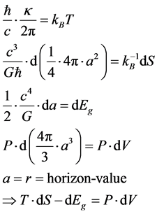 (2)
(2)
The last equation of Equation (2) below is what will be reviewed, using the lens of having the pressure, small, and constant. Using the idea that pressure is the negative of density in inflation.
2. Reviewing What to Do with Pressure, Using the Ideas of Inflation
We use that pressure is the negative of density as to how to power inflation, as well as Equation (2). In doing so the start of the analysis, is to use Equation (3) below to parameterize pressure and density due to B fields. By [2]
 (3)
(3)
This has a positive value only if
 (4)
(4)
For fidelity with inflation, we wish to have the magnetic field bounded as given in Equation (4), i.e. Equation (4) is necessary for negative pressure, which is only true, initially, if the density is positive, which puts in a major constraint upon the background B field. i.e. we can argue that there would be likely by the electro weak regime, an increase of the magnetic field, probably due to the synthesis of plasmas leading to E and B field generation, but that there would need to be a critical B field strength. so as to make Equation (3) and Equation (4) consistent with inflation. In order to evaluate Equation (2) so as to extract an initial inflationary temperature, we will be considering a critical B field strength relevant as to initial negative pressure which could affect the strength of GW propagation. Finally in the end which wish to have Equation (3) and Equation (4) as consistent with the Davis [3] value of vacuum energy density which we write as
 (5)
(5)
Davis rules out quintessence (varying the cosmological constant over time) whereas in our application, we will be asking that our value of Equation (5) is consistent with the High Z super nova search team graph given in Figure 1 [4] . In essence, that means that our calculations as to density would have to reflect the physics of [3] and [5] as given by.
 (6)
(6)
The following bound would have to be adhered to, if the cyclic model of the universe as given by Steinhardt and others held [6] then the frequency as given in Equation (4) would be related to the vacuum energy [6] [7]

Figure 1. (distance/10 pc) so the most distant SN on this plot is at about 7.6 billion pc.) From [4] . This graph tends to suggest that the cosmological constant is a constant, not variable.
 (7)
(7)
One could realistically that that then, according to Equation (4) and Equation (7) that for a small cosmological constant, that the frequency associated due to an early universe magnetic field would be relatively high. i.e. in doing so, this would set the stage for what comes next, namely setting the frequency of radiation from a first principle fashion which will lead to several goals:
a) Getting temperature dependence, as affected by the frequency,  (NLED used explicitly here)
b) Making a full analysis of the impact of the last equation of the grouping of Equation (2), taking into account entropy, and a comparison of energy, as will be explained, in our Equation (12) as given below Figure 1 on the next page.
c) A balance of entropy, versus energy will be entertained and used to explain how to contribute to the strength of a signal. i.e. our outrageous suggestion is that if we understand negative pressure that we will be in turn able to discuss, up to a point, the strain, h, of relic GW. This last topic will be in the latter part of this document, as part of the conclusion. This, also in part will be seen in a rigorous treatment of [8] which has similarities to what is given in [9]
 (8)
(8)
From here, we use the following to isolate out the term h, strain, as can be seen in [8]
 (9)
(9)
In doing this approximation, we then will read the trace of T (in Equation (8)) as reading as, in our appro- ximation which has issues and motivation given in [9] but similar to the Davis article [3]
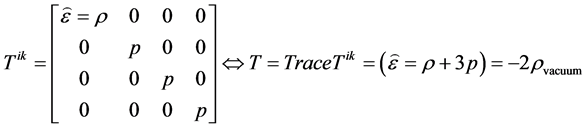 (10)
(10)
If so, then one has a simple expression for h, as given by
 (11)
(11)
We will from here, calculate strain h, and then set up how to evaluate the initial temperature
3. Reviewing What to Do with a Minimum Negative Pressure, Its Importance, and Equation 2 When Examining the Strength of Relic GW
To begin with, we make the following approximation as adopted and modified from [1]
 (12)
(12)
This above is the temperature, with the S as a measure of initial entropy. If the frequencies in the beginning of this expression are the same as in the density  with the density as given by Equation (3) then one is observing
 (13)
(13)
Secondly, we can then look at the strength of the strain as
 (14)
(14)
Next, we will consider the input frequencies to be used in this situation.
4. Frequency Input into Equation (13) and Equation (14) as Given in by Equation (19)
The basic working tools come from [10] with the following formulations, first of all, the spectral index, defined by, if 
 (15)
(15)
This should be compared with the e fold equation, as given by
 (16)
(16)
We should note that there are models of e fold which are as low as 60 as given in [1] , and that the value of 70 is put in as a convenience, but not necessarily true. The figure of 70 gives a very small value to the initial wavelength, which is put in for illustrative purposes. The very small wavelength makes our point about Equation (18) easier to fathom, i.e. the comparative largeness of the potential energy, which changes dramatically with expansion of the universe, during inflation.
Equation (16) is used in tandem with the potential in question to be rendered as
 (17)
(17)
Furthermore, the potential, reconstructed, is to be compared to a frequency via using the re constructed inflation potential value.
 (18)
(18)
i.e. after constructing the potential, via Equation (18), obtaining an initial wave function is given by
 (19)
(19)
This initial value of inflation is related to Equation (16) above via a final value damped by Equation (16) via
 (20)
(20)
The frequency, initially, is about 2 orders of magnitude larger than the Planck frequency as given below
 (21)
(21)
The reasons for such statements and their consequences will be the subject of the following article.
5. Showing How to Reconstruct the Potential (Energy)
We write, most likely, that the initial time step is of the order of
 (22)
(22)
Keep in mind that in standard cosmology inflation starts around 10−35 seconds after the big bang and ends around 10−32 seconds after the big bang. The Planck time picked in Equation (22) is before the initiation of inflation, but is picked if we view the potential energy as an emergent phenomenon which starts at the smallest interval of time itself. We pick the minimum time step as smaller than the onset of inflation and specify a small delay, between 10−44 seconds, to 10−35 seconds. i.e. for more than 4 dimensions there should be an emergent potential energy phenomenon, which starts taking effect in 10−44 seconds and which creates in 4 dimensions the potential energy as a non-zero contribution in 10−35 seconds. We will in a future article, specifically outline the mechanism for this difference in start times between 5 and higher dimensional representations of the potential energy beginning as an emergent field phenomenon, and having a non-zero 4 dimensional contribution as taking effect in 10−35 seconds.
If one takes the Calibi-Yau string theory [11] approach to higher dimensions, the initiation of potential energy in more than 4 dimensions is in a sense equivalent to string theory treatment of the higher dimensions as very small. Small but not insignificant, as what will become very apparent in our future publication on this matter.
For now on, we will stick with the convention picked in Equation (22) and leave its full elaboration as a follow up to this article.
In doing so, we will fix the inflaton as an emergent field which starts making its contribution in 10−44 seconds.
Using this convention, we have the following, namely
The coefficients of the potential to be worked with in Equation (17)
 (23)
(23)
We set the initial inflaton via the equation assuming that  is a constant, that according to [1]
 (24)
(24)
This assumes that
 (25)
(25)
So then that we can use a quadratic value, for a potential which is V given by
 (26)
(26)
If we pick , and
, and
 (27)
(27)
For initial conditions, then Equation (16) will yield
 (28)
(28)
To first approximation, the above is giving an initial frequency of
 (29)
(29)
The relevant wavelength is, then approximately 1/1041 Hz, or
 (30)
(30)
We will next comment upon the consequences of Eq. (30) and the aftermath.
6. Avoiding the Bicep 2 Disaster and Falsifiability of the Possibility of More than 2 Polarization States for Gravitational Waves (The Search for an Alternative to General Relativity, Experimentally Tested)
In our choice of frequencies, it is most important to look at the requirements for single source generation of gravitational waves, as can be ascertained by [12] which puts in strict observational restrictions as to what can be observed, as to avoid the dust generated multiple source, very noisy stochastic background which was the undoing of Bicep 2. This means paying attention to the requirements given as of [13] - [16] as to suitable frequencies as for Equation (28). Furthermore, Equation (28) should be carefully investigated as to answer the question raised by Corda in [13] as to if there are more than 2 polarization states for gravitational waves, which would indicate a scalar-tensor tensor gravitational theory for cosmology in place of general relativity. If there is just 2 polarization states, as stated in [13] then of course we can stick with traditional General relativity. This means though that in our work, the detected frequencies are what we want, and not due to multiple sources in a stochastic background. Furthermore, since we are referencing nonlinear electrodynamics, this leads to the next section. While assuming that the analysis given in [17] holds
7. Application to Non Linear Electrodynamics, NLED, to Various Astrophysical Phenomena
In reference [18] , we have reference to a phenomenon which we hope to avoid, namely as seen in
(section 3) PREPARING THE DATA:
In this paper we analyze the publicly available WMAP data after correction for Galactic foregrounds. We consider data from the V and W frequency bands only since these are less likely to be contaminated by residual foregrounds. The maps from the different channels are co added using inverse noise-weighting.
What we are trying to do is, to use the methodology of [18] to avoid contamination of our probable signals for primordial gravitational waves from foreground contamination which is due to galaxies. The signal contamination as illustrated in [15] [16] is what lead to Bicep 2 data being considered hopelessly stochastic, which is indistinguishable from multiple sources of later non primordial gravitational waves.
Corda in [19] has further refined the problem by a so called biometric theory of gravity in which his statement of the polarization phenomenon [13] may be linked to our Equation (3) being correctly evaluated. But that in turn means being careful of the problem which was brought up by [20] in which Non Linear Electrodynamics [NLED] is not the same as that of General relativity. The example of Questa in [20] is for neutron stars, and for a physical set up which involves admittedly a different theory, than General relativity, but in turn, it means that what is stated for the permissible values of the magnetic field as pertinent to Equation (3) have to be given in such a way that the Non Linear Electrodynamic effects affecting gravitational waves will have to be, as given in the [20] neatly bifurcated from those of General Relativity.
We very likely will be in the situation in which NLED phenomenon in the very early universe has its own contribution to gravitational waves, and that contribution for much the same reason as given in [20] will be apportioned with the influence of General Relativity. How we apportion the relative contributions of NLED and General Relativity will likely be crucial in determining the validity of the Corda suppositions given in both [13] and in [19] , in tests for the confirmation of if General Relativity should be considered the definitive theory for gravitational physics in Cosmology.
8. Conclusions
Our conclusion is to look at the given frequency, and then the wavelength, taking into account the gigantic expansion from inflation, i.e. the 60 to 70 e fold expansion given by inflation. Reference [1] gives us via inflation that Equation (16) yields, say for Gravity waves, the values
 (31)
(31)
These values, due to an E fold value given through Equation (16) allow us to state that inflation physics gives us incredibly high initial GW frequencies, which will yield new visas as to how to look at relic GW [1] [2] The strain to be considered comes out to , to be observed, and if the entropy, initially is
 (32)
(32)
 (33)
(33)
Equation (33) drops if the initial entropy is greater than the value given in Equation (32), which has implications the author will be reviewing.
Our specific future work, will be divided between revisiting the issue given in [20] as it applies to early universe primordially generated gravitational waves. In addition as stated before
We will in a future article, specifically outline the mechanism for this difference in start times between 5 and higher dimensional representations of the potential energy beginning as an emergent field phenomenon, and having a non-zero 4 dimensional contribution as taking effect in 10−35 seconds.
It is the reasoned conclusion of the author that these two issues are in part intertwined, and that these two issues will be part of a future publication where we examine both, and hope to ascribe the origins of both Non Linear Electrodynamic contributions to gravity, and what is given in the quote above, as part of additional physical investigation into the origins of the CMBR, so as to avoid the problems given in [15] [16] which wrecked Bicep 2.
Acknowledgements
This work is supported in part by National Nature Science Foundation of China grant No. 11375279.
Cite this paper
Andrew WalcottBeckwith, (2016) Thermodynamics and the Energy of Gravity Waves, GW’s, as a Consequence of Non Linear Electrodynamics, NLED, Leading to an Initial Temperature and Strain h for Gravity Waves, GW, at the Start of Inflation. Journal of High Energy Physics, Gravitation and Cosmology,02,98-105. doi: 10.4236/jhepgc.2016.21011
References
- 1. Padmanabhan, T. (2011) Lessons from Classical Gravity about the Quantum Structure of Space-Time. Journal of Physics: Conference Series, 306, Article ID: 012001. http://iopscience.iop.org/1742-6596/306/1/012001/pdf/1742-6596_306_1_012001.pdf http://dx.doi.org/10.1088/1742-6596/306/1/012001
- 2. Camara, C.S., de Garcia Maia, M.R., Carvalho, J.C. and Lima, J.A.S. (2004) Nonsingular FRW Cosmology and Non Linear Dynamics. Arxiv astro-ph/0402311 Version 1, Feb 12.
- 3. Davis, E.W. (2009) Review of Gravity Control. In: Millis, M. and Davis, E., Eds., Frontiers of Propulsion Science, (Progress in Astronautics and Aeronautics), AIAA, Volume 227, 175-228.
- 4. Riess, A.G., Filippenko, A.V., Li, W.D. and Schmidt, B.P. (1999) Is There an Indication of Evolution of Type Ia Supernovae from Their Rise Times? The Astronomical Journal, 118, 2668-2674. http://iopscience.iop.org/1538-3881/118/6/2668/fulltext/
- 5. Carmeli, M. and Kuzmenko, T. (2001) Value of the Cosmological Constant: Theory versus Experiment. http://www.aldebaran.cz/studium/vnp/docs/Lambda.pdf
- 6. Steinhardt, P.J. and Turok, N. (2002) A Cyclic Model of the Universe. Science, 296, 1436-1439. http://dx.doi.org/10.1126/science.1070462
- 7. Rugh, S. and Zinkernagel, H. (2001) The Quantum Vacuum and the Cosmological Constant Problem. http://philsci-archive.pitt.edu/398/
- 8. Maggiorie, M. (2008) Gravitational Waves, Volume 1, Theory and Experiments. Oxford University Press, Oxford, UK.
- 9. Lehmkuhl, D. (2011) Mass-Energy-Momentum: Only There Because of Spacetime? British Journal for the Philosophy of Science, 62, 453-488. http://dx.doi.org/10.1093/bjps/axr003
- 10. Padmanabhan, T. (2005) Understanding Our Universe: Current Status and Open Issues. arXiv: gr-qc/0503107v1. http://arxiv.org/pdf/gr-qc/0503107.pdf
- 11. Greene, B. (1997) String Theory on Calabi-Yau Manifolds. http://arxiv.org/abs/hep-th/9702155
- 12. Van Den Broeck, C. (2015) Gravitational Wave Searches with Advanced LIGO and Advanced Virgo. http://arxiv.org/abs/1505.04621
- 13. Corda, C. (2009) Interferometric Detection of Gravitational Waves: The Definitive Test for General Relativity. International Journal of Modern Physics D, 18, 2275-2282. http://arxiv.org/abs/0905.2502; http://dx.doi.org/10.1142/S0218271809015904
- 14. Das, S., Mukherje, S. and Souradeep, T. (2015) Revised Cosmological Parameters after BICEP 2 and BOSS. http://arxiv.org/abs/1406.0857
- 15. Cowen, R. (2015) Gravitational Waves Discovery Now Officially Dead; Combined Data from South Pole Experiment BICEP2 and Planck Probe Point to Galactic Dust as Confounding Signal. http://www.nature.com/news/gravitational-waves-discovery-now-officially-dead-1.16830
- 16. Cowen, R. (2014) Full-Galaxy Dust Map Muddles Search for Gravitational Waves. http://www.nature.com/news/full-galaxy-dust-map-muddles-search-for-gravitational-waves-1.15975
- 17. Beckwith, A. (in press) Geddanken Experiment for Degree of Flatness, or Lack of, in Early Universe Conditions. Accepted for publication, JHEPGC. http://vixra.org/abs/1510.0108
- 18. Hansen, F.K., Banday, A.J. and Gorski, K.M. (2004) Testing the Cosmological Principle of Isotropy: Local Power Spectrum Estimates of the WMAP Data. arXiv: astro-ph/0404206v1. http://120.52.73.75/arxiv.org/pdf/astro-ph/0404206v1.pdf
- 19. Corda, C. (2007) A Longitudinal Component in Massive Gravitational Waves Arising from a Bimetric Theory of Gravity. Astroparticle Physics, 28, 247-250. http://dx.doi.org/10.1016/j.astropartphys.2007.05.009
- 20. Cuesta, H.J.M. and Salim, J.M. (2004) Non Linear Electrodynamics and the Gravitational Redshift of Highly Magnetized Neutron Stars. Monthly Notices of the Royal Astronomical Society, 354, L.55-L.59.