Received 9 December 2015; accepted 23 January 2016; published 27 January 2016

ABSTRACT

In this paper, we consider an unknown source problem for the modified Helmholtz equation. The Tikhonov regularization method in Hilbert scales is extended to deal with ill-posedness of the problem. An a priori strategy and an a posteriori choice rule have been present to obtain the regularization parameter and corresponding error estimates have been obtained. The smoothness parameter and the a priori bound of exact solution are not needed for the a posteriori choice rule. Numerical results are presented to show the stability and effectiveness of the method.

Keywords:

Ill-Posed Problem, Unknown Source, Regularization Method, Discrepancy Principle in Hilbert Scales

1. Introduction

A variety of important problems in science and engineering involve the solution to the modified Helmholtz equation, e.g., in implicit marching schemes for the heat equation, in Debye-Huckel theory, and in the linearization of the Poisson-Boltzmann equation [1] - [5] . In this paper, we consider the following problem of determining an unknown source which depends only on one variable for the modified Helmholtz equation [6] :

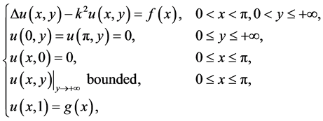(1)

where is the unknown source and is the supplementary condition and the constant is the wave number. Our purpose is to identify the source term from the input data. This

problem is called the inverse source problem. In practice, the data at are often obtained on the basis of reading of physical instrument. So only a perturbed data can be obtained. We assume that the exact and measured data satisfy

(2)

where denotes the noise level, denotes the―norm.

Inverse source problems arise in many branches of science and engineering, e.g., heat conduction, crack identification electromagnetic theory, geophysical prospecting and pollutant detection. The main difficulty of these problems is that they are ill-posed (the solution, if it exists, does not depend continuously on the data). Thus, the numerical simulation is very difficult and some special regularization is required. Many papers have presented the mathematical analysis and efficient algorithms of these problems. The uniqueness and conditional stability results for these problems can be found in [7] - [12] . Some numerical reconstruction schemes can be found in [13] - [23] .

Up to now, only a few papers for identifying the unknown source on the modified Helmholtz equation have been reported. In [1] , an integral equation method has been proposed and a simplified Tikhonov regularization has been presented in [6] . In this paper, we will use the Tikhonov regularization method to solve the problem (1). Unlike the one in [6] , a different Tikhonov functional will be used and we show that the regularization parameter can be chosen by a discrepancy principle in Hilbert scales which is proposed by Neubauer [24] and better convergence rates have been obtained. Moreover, the smoothness parameter of the exact solution is not needed for the new method.

This paper is organized as follows. In Section 2, we will give the method to construct approximate solution. The choices of the regularization parameter and corresponding convergence results will be found in Section 3. Some numerical results are given in Section 4 to show the effectiveness of the new method.

2. The Tikhonov Regularization Method

Let, it is well known that is an orthonormal basis in, i.e.,

(3)

where is the Kronecher symbol. So for any, we can write, where

(4)

It is easy to derive a solution of problem (1) by the method of separation of variables [6]

(5)

where

(6)

Note that the exact data must decay faster than the rate. As for the measured data function is only in, we cannot expect that it possess such a decay property. So some special regularization methods are required. In the following, we apply the Tikhonov regularization method in Hilbert scales to reconstruct a new function from the perturbed data and will be used as an approximation of f. It is well known that for any ill-posed problems an a priori bound assumption for the exact solution is needed and necessary. In this paper, we assume the following a priori bound holds:

(7)

where is a constant and denotes a slightly different norm from the one in [25] which is defined by:

(8)

where

(9)

We let be the minimizer of the Tikhonov functional

(10)

where is a regularization parameter and q is a positive real number. The real number is going to occur throughout this paper and will be denoted by.

If we let, then we can derive that satisfy

(11)

So we have

(12)

Which means that

(13)

Then the approximate solution can be given as

(14)

Lemma 1. For any, we have

(15)

Lemma 2. [26] For, we have

(16)

Lemma 3.

(17)

where is the unique minimizer of (10) with g instead of.

Proof.

(18)

The proposition follows by applying (16) with b replaced by.

Lemma 4.

(19)

where

(20)

Proof. With the representation

(21)

and Lemma 1, we have

(22)

3. The Choices of Regularization Parameter a and Convergence Results

In this section, we consider the choices of the regularization parameter. An a priori strategy and an a posteriori choice rule will be given. Under each choice of the regularization parameter, the convergence estimate can be obtained.

3.1. The a Priori Choice Rule

Take

(23)

we can obtain the following theorem.

Theorem 5. If (2) holds and (7) holds with, is defined by (14) and (23), then

(24)

Proof. With Lemma 3, Lemma 4 and (23) we obtain

(25)

Moreover, by using Hölder inequality, we have

(26)

Formulae (8) implies that

(27)

The assertion of the Lemma follows from (25)-(27).

3.2. The a Posteriori Choice Rule

For any, we define

(28)

It is apparent that the function is continuous and strictly increasing on and

(29)

So we can get the following lemma

Lemma 6. Let g, and satisfy (2) and

(30)

for some. Then there is a unique such that

(31)

In the following, we denote the unique determined in (31) by. In the next lemma, we consider the behavior of.

Lemma 7. Let g, and satisfy (2) and (30) for.

a)

(32)

b)

(33)

where

(34)

Proof.

a) Let

(35)

then

(36)

b)

(37)

then from Lemma 1

(38)

The rest follows from a).

Theorem 8. Suppose that the conditions (2) and (30) hold, the condition (7) hold with, is defined by (14) and (31), then

(39)

Proof. By using the triangle inequality we know

(40)

So, in terms of Equations (17), (19) and (33), we have

(41)

From (26),

(42)

Combining (41) and (42), we obtain

(43)

The assertion of the theorem follows from (27).

4. Numerical Tests

In this section, we present some numerical tests to check the effectiveness of the method. The discretization knots are. We first get the datum representing values of, and then obtain the perturbation datum as following

(44)

where are generated by Function in Matlab. Because the error satisfies the uniform distribution in this paper, so we let

in practical computing. The relative errors are measured by the weighted -norms defined as follows:

(45)

All tests are computed by using Matlab and we will also compare the method (M1) with the method in [6] (M2, notate the approximate function as). The perturbed data are given by

(46)

where are generated by function in Matlab.

Example [6] It is easy to see that the function and the function are the exact solutions of the problem (1) for any natural number n. In these cases, the condition (7) hold for any. So we have. Firstly, we exhibit influence of various p and N on ac- curacy of numerical solution. The relative errors have been shown in Table 1 with, and fixed. We can see that when N increases and decreases, the relative errors become smaller and when q increases, the rates of convergence become larger.

In Table 2, we give a numerical comparison between M1 and M2 with fixed,. The relative errors are given in Table 2, we can see that the results of M1 are much better than M2.

5. Conclusion

We have proposed a new method to identify the unknown source in the modified Helmholtz equation. Theoretical analysis as well as experience from computations indicates that the proposed method works well.

Acknowledgements

The project is supported by the National Natural Science Foundation of China (No. 11201085).

Cite this paper

LeiYou,ZhiLi,JuangHuang,AihuaDu, (2016) The Tikhonov Regularization Method in Hilbert Scales for Determining the Unknown Source for the Modified Helmholtz Equation. Journal of Applied Mathematics and Physics,04,140-148. doi: 10.4236/jamp.2016.41017

References

- 1. Cheng, H., Huang J. and Leiterman, T.J. (2006) An Adaptive Fast Solver for the Modified Helmholtz equation in Two Dimensions. Journal of Computational Physics, 211, 616-637.
http://dx.doi.org/10.1016/j.jcp.2005.06.006 - 2. Juffer, A.è.H., Botta, E.F.F., van Keulen, B.A.M., van der Ploeg, A. and Berendsen, H.J.C. (1991) The Electric Potential of a Macromolecule in a Solvent: A Fundamental Approach. Journal of Computational Physics, 97, 144-171.
http://dx.doi.org/10.1016/0021-9991(91)90043-K - 3. Kropinski, M.C.A. and Quaife, B.D. (2011) Fast Integral Equation Methods for the Modified Helmholtz Equation. Journal of Computational Physics, 230, 425-434.
http://dx.doi.org/10.1016/j.jcp.2010.09.030 - 4. Liang, J. and Subramaniam, S. (1997) Computation of Molecular Electrostatics with Boundary Element Methods. Biophysical Journal, 73, 1830-1841.
http://dx.doi.org/10.1016/S0006-3495(97)78213-4 - 5. Russel, W.B., Saville, D.A. and Schowalter, W.R. (1991) Colloidal Dispersions. Cambridge University Press, Cambridge.
- 6. Fan, Y., Guo, H.Z. and Li, X.X. (2011) The Simplified Tikhonov Regularization Method for Identifying the Unknown Source for the Modified Helmholtz Equation. Mathematical Problems in Engineering, 2011.
- 7. Cannon, J.R. and DuChateau, P. (1998) Structural Identification of an Unknown Source Term in a Heat Equation. Inverse Problems, 14, 535.
http://dx.doi.org/10.1088/0266-5611/14/3/010 - 8. Cannon, J.R. and Perez-Esteva, S. (1991) Uniqueness and Stability of 3d Heat Sources. Inverse Problems, 7, 57.
http://dx.doi.org/10.1088/0266-5611/7/1/006 - 9. Choulli, M. and Yamamoto, M. (2004) Conditional Stability in Determining a Heat Source. Journal of Inverse and Ill-Posed Problems, 12, 233-243.
http://dx.doi.org/10.1515/1569394042215856 - 10. El Badia, A. and Ha-Duong, T. (2002) On an Inverse Source Problem for the Heat Equation. Application to a Pollution Detection Problem. Journal of Inverse and Ill-Posed Problems, 10, 585-600.
http://dx.doi.org/10.1515/jiip.2002.10.6.585 - 11. Li, G.S. (2006) Data Compatibility and Conditional Stability for an Inverse Source Problem in the Heat Equation. Applied Mathematics and Computation, 173, 566-581.
http://dx.doi.org/10.1016/j.amc.2005.04.053 - 12. Yamamoto, M. (1993) Conditional Stability in Determination of Force Terms of Heat Equations in a Rectangle. Mathematical and Computer Modelling, 18, 79-88.
http://dx.doi.org/10.1016/0895-7177(93)90081-9 - 13. Burykin, A.A. and Denisov, A.M. (1997) Determination of the Unknown Sources in the Heat-Conduction Equation. Computational Mathematics and Modeling, 8, 309-313.
http://dx.doi.org/10.1007/BF02404048 - 14. Dou, F.F., Fu, C.L. and Yang, F.L. (2009) Optimal Error Bound and Fourier Regularization for Identifying an Unknown Source in the Heat Equation. Journal of Computational and Applied Mathematics, 230, 728-737.
http://dx.doi.org/10.1016/j.cam.2009.01.008 - 15. Farcas, A. and Lesnic, D. (2006) The Boundary-Element Method for the Determination of a Heat Source Dependent on One Variable. Journal of Engineering Mathematics, 54, 375-388.
http://dx.doi.org/10.1007/s10665-005-9023-0 - 16. Ling, L., Yamamoto, M., Hon, Y.C. and Takeuchi, T. (2006) Identification of Source Locations in Two-Dimensional Heat Equations. Inverse Problems, 22, 1289-1305.
http://dx.doi.org/10.1088/0266-5611/22/4/011 - 17. Park, H.M. and Chung, J.S. (2002) A Sequential Method of Solving Inverse Natural Convection Problems. Inverse Problems, 18, 529-546.
http://dx.doi.org/10.1088/0266-5611/18/3/302 - 18. Ryabenkii, V.S., Tsynkov, S.V. and Utyuzhnikov, S.V. (2007) Inverse Source Problem and Active Shielding for Composite Domains. Applied Mathematics Letters, 20, 511-515.
http://dx.doi.org/10.1016/j.aml.2006.05.019 - 19. Yan, L., Fu, C.L. and Yang, F.L. (2008) The Method of Fundamental Solutions for the Inverse Heat Source Problem. Engineering Analysis with Boundary Elements, 32, 216-222.
http://dx.doi.org/10.1016/j.enganabound.2007.08.002 - 20. Yan, L., Yang, F.L. and Fu, C.L. (2009) A Meshless Method for Solving an Inverse Spacewise-Dependent Heat Source Problem. Journal of Computational Physics, 228, 123-136.
http://dx.doi.org/10.1016/j.jcp.2008.09.001 - 21. Yang, F. (2011) The Truncation Method for Identifying an Unknown Source in the Poisson Equation. Applied Mathematics and Computation, 22, 9334-9339.
http://dx.doi.org/10.1016/j.amc.2011.04.017 - 22. Yang, F. and Fu, C.L. (2012) The Modified Regularization Method for Identifying the Unknown Source on Poisson Equation. Applied Mathematical Modelling, 2, 756-763.
http://dx.doi.org/10.1016/j.apm.2011.07.008 - 23. Yi, Z. and Murio, D.A. (2004) Source Term Identification in 1-D IHCP. Computers & Mathematics with Applications, 47, 1921-1933.
http://dx.doi.org/10.1016/j.camwa.2002.11.025 - 24. Neubauer, A. (1988) An a Posteriori Parameter Choice for Tikhonov Regularization in Hilbert Scales Leading to Optimal Convergence Rates. SIAM Journal on Numerical Analysis, 25, 1313-1326.
http://dx.doi.org/10.1137/0725074 - 25. Kirsch, A. (1996) An Introduction to the Mathematical Theory of Inverse Problems. Springer-Verlag, New York.
http://dx.doi.org/10.1007/978-1-4612-5338-9 - 26. Natterer, F. (1984) Error Bounds for Tikhonov Regularization in Hilbert Scales. Applicable Analysis, 18, 29-37.
http://dx.doi.org/10.1080/00036818408839508