Theoretical Economics Letters
Vol.2 No.3(2012), Article ID:21500,4 pages DOI:10.4236/tel.2012.23053
A Biased Expectation Equilibrium in Indeterminate DSGE Models*
School of Commerce, Meiji University, Tokyo, Japan
Email: tamegawa@kisc.meiji.ac.jp
Received March 2, 2012; revised April 4, 2012; accepted May 7, 2012
Keywords: DSGE Modeling; Rational Expectations Model; Indeterminacy
ABSTRACT
The aim of this article is to introduce a solution method for an indeterminate dynamic stochastic general equilibrium (DSGE) model. The method uses the concept of a biased expectation equilibrium, which is defined in this paper and means that expectations of certain variable are mechanically biased against those that would be rational. Our method should be particularly useful in terms of empirical estimation using DSGE models, because it will allow researchers to estimate how much agents’ expectations are biased in the case where a model has indeterminacy.
1. Introduction
There are many methods available for computing the saddle path of a linear rational expectations model. However, a model of this sort can nevertheless be in a condition of indeterminacy. For example, it is well known that in a simple New Keynesian model, comprised of the consumption Euler equation, the New Keynesian Phillips curve, and a monetary policy rule, equilibrium is indeterminate if the monetary policy is accommodative of inflation; for example, see Leeper [1].
As surveyed in Fernández-Villaverde [2], the methods for estimating DSGE models have been developed and many empirical studies, such as that of Smets and Wouters [3] have been conducted. Notably, most of these studies assume that an economy is always on a saddle path, although an economy can have a possibility of indeterminacy (The exception is Lubik and Schorfheide [4]. They evaluate the US economy using a simple New Keynesian model that allows for indeterminacy). However, this assumption may be restrictive It is hence useful to develop a method that can handle indeterminacy, especially for empirical research programs. Furthermore, with such a method, the forecasting performance of the DSGE-VAR model, which is introduced by Del Negro and Schorfheide [5], would be improved.
To handle indeterminacy, this article introduces 1) a biased expectations equilibrium in which certain variables’ expectations are biased against rational expectations and 2) a method of computing that equilibrium. Lubik and Schorfheide [6] have demonstrated how to handle indeterminacy through exogenous sunspot shocks, based on Sims [7]. Our approach is different from theirs in that the path of economic variables is here determined through subjective expectations that may be independent of the underlying structural model. This paper simply expresses “subjective expectations” as a situation under which expectations are mechanically biased with respect to rational expectations.
Our paper is organized as follows. Section 2 sets a linear rational expectations model. Section 3 introduces the definition of a biased expectation equilibrium and shows how to compute a biased equilibrium by employing subjective expectations. Section 4 constructs a simple New Keynesian model, and we apply our method to it.
2. Settings of the Model
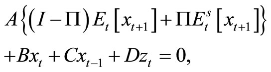
Consider the following linear rational expectations model:
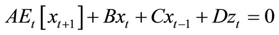 , (1)
, (1)
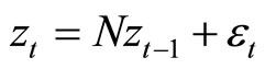 ,
,  for all
 where
where  denotes a vector of endogenous variables that comprise k state variables and n jump variables, and
  represents a vector of the exogenous variables. Then, what we are looking for is the following expression:
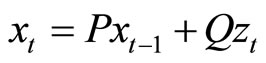 , (2)
, (2)
Note that in these settings, the lagged jump variables are taken as state variables.1 Substituting Equation (2) into Equation (1), the following conditions are obtained:
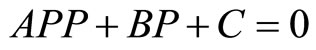 , (3)
, (3)
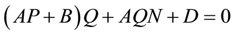 , (4)
, (4)
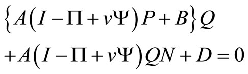
The matrix quadratic Equation (3) can be used to check whether the solution is none, indeterminate, or unique by using the following matrices:
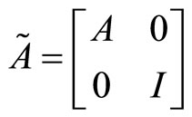
and
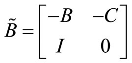 where I represents the identity matrix. To solve Equation (3), we apply QZ decomposition to
  and
and . This decomposition yields upper triangular matrices S and T and orthogonal matrices
  and Z, such that
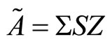
and
 .
.
This decomposition can be arranged such that the absolute ratio of diagonal entries of S and T (that is ), is in ascending order. If the number of the ratio exceeding one denoted by r is equal to n, the model has a saddle path. On the other hand, if
 , the solution is indeterminate.2
By QZ decomposition and counting r, the following restrictions for  are obtained:
 (5)
(5)
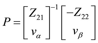
where Z21 and Z22 denote block matrices of size . If
. If , then P can be computed as:
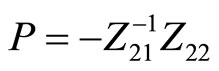 (6)
(6)
If , then P cannot be determined uniquely and this case (indeterminacy) will be explained in the next section.
The matrix Q is calculated from (4) as follows
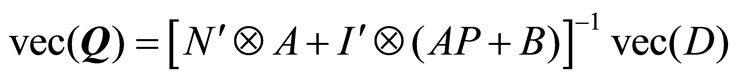 where “
 ” operator denotes column-wise vectorization.
3. A Biased Expectations Equilibrium
Assume the indeterminate economy, that is,
 . In this case, P cannot be uniquely obtained. Therefore, additional restrictions for P are needed. To set these restrictions, we assume the existence of forecasters who form expectations of certain variables based on their subjective knowledge. Furthermore, this paper assumes that agents in the economy use subjective expectation in their decision-making. This paper simply assumes that the subjective expectation is expressed as a situation under which it there is mechanical bias against rational expectations.
3.1. Definition
This section defines a biased expectation equilibrium. To do this, we assume that subjective expectations are related to rational expectations as follows. Letting  be the ith element of
 ,
,
 (7)
(7)
where the “ ” operator is the operator of subjective expectations. Suppose that this forecaster always forms the biased expectations that are represented by the scalar
 . Assume that the biased expectations of the ith element of
  are formed in the following manner (for example, by traditional macro-econometric models):
 , (8)
, (8)
where  denotes an
  dimensional row vector. Note that Equation (8) may be independent of the underlying economic structure, and that if
 , subjective expectation reduces to adaptive expectation.
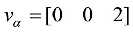
Next note that p forecasts, expressed as Equation (8), are required to compute P. In order to choose the variables predicted by the forecasters from , define the choice matrix v of size
  such that for each row, the ith column takes one if the ith variable of
  is to be forecasted and zero otherwise. For example, if
  and the forecasters predict the first and the second variable of
 , then
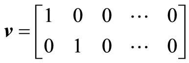 .
.
From this choice matrix, the following equation is obtained
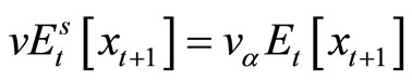 (9)
(9)
where  is a
is a  matrix such that one in v is replaced by
 . Furthermore, v and Equation (8) yield
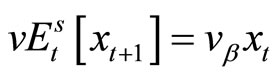 , (10)
where  represents a
  matrix such that each row is
 . For expectations other than
 , it is assumed that agents can form rational expectations. Here, we define a biased expectations equilibrium path as follows.
3.2. Definition: A Biased Expectations Equilibrium
Suppose . We call the sequence
  a biased expectations equilibrium path if it satisfies Equations (1), (9), and (10).
3.3. Computation Method
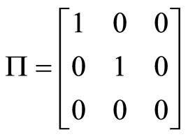
A biased expectations equilibrium path can be easily computed as follows. If , then the model represented by Equation (1) can be replaced by
 (11)
(11)
where  represents a
  matrix such that the ith diagonal element is one if the ith variable of
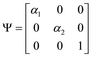
  is to be forecasted and zero otherwise. To facilitate computation, define
  as an
as an  diagonal matrix such that the ith diagonal element is
  if the ith variable of
  is to be forecasted and one otherwise. The off-diagonal entries of
  and
and  are zero. In the example with
  and
and , if
, if ,
,  , and the forecasted variables are the first and second elements of
 ,
,
and
In this case, noting
 Equations (3) and (4) are replaced by
 (12)
(12)
 (13)
(13)
Equations (2), (9), and (10) yield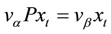 . Therefore, the following equations are obtained:
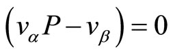 . (14)
Using the restrictions that are implied by Equation (11), we can compute the unique P as follows:
 . (15)
where  and
and  are obtained by the QZ decomposition of
  in which A is replaced by
 , and
, and . Note that to obtain a biased expectation equilibrium, it is needed that the underlying model has
  under this replaced
 .
.
4. Example
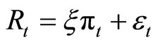
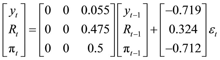
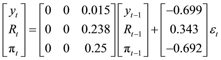
This section provides examples of the application of our method to an indeterminate economy. Consider the following simple New Keynesian Model described by
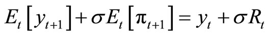 ,
,
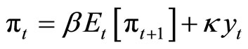 ,
,
 where
where  denotes the output,
  the inflation, and
  the nominal interest rate. All variables are deviations from the steady state;
  denotes a monetary policy shock, and
  for all
 . Using the notation of the model (1),
 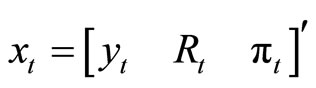 and
and . For the coefficients matrices,
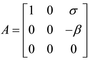 ,
, 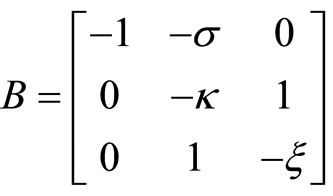 ,
, 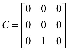 and
and
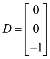 .
.
It is well known that if  (the Taylor principle), the model has a unique path. Note that in this case P is the zero matrix, and if
 , the solution is indeterminate.
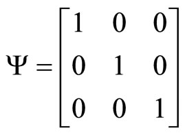
Suppose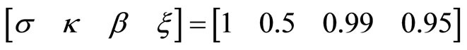 . In this case, we have
 . Further, assume that
 ,
,
 and
and
 .
.
Note that  implies that agents’ expectations are adaptive. These imply that
 ,
,
 and
and
 .
.
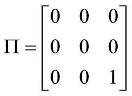
Applying our method, we obtain
 Next, consider that the forecasters overestimate expected inflation in the sense of
 , which implies
in the above settings.3 In this case,
 .
.
This result implies that if the forecasters’ estimates are overshot, then the effect of the monetary policy will be mitigated.
5. Final Remarks
In this paper, we presented a way to handle indeterminacy in DSGE models by introducing a biased expectations equilibrium in which certain variables’ expectations are biased against rational expectations. We then introduced a method for such an equilibrium. The method is particularly useful in terms of the empirical estimation of DSGE models, because in an indeterminate economy, researchers can estimate how much agents’ expectations are biased.
Whether a biased equilibrium in an indeterminate economy as defined in this paper is actually valid is an empirical matter and a task for future research.
REFERENCES
- E. M. Leeper, “Equilibria under ‘Active’ and ‘Passive’ Monetary and Fiscal Policies,” Journal of Monetary Economics, Vol. 27, No. 1, 1991, pp. 129-147. doi:10.1016/0304-3932(91)90007-B
- J. Fernández-Villaverde, “The Econometrics of DSGE Models,” NBER Working Paper, No. 14677, 2009.
- F. Smets and R. Wouters, “An Estimated Dynamic Stochastic General Equilibrium Model of the Euro Area,” Journal of the European Economic Association, Vol. 20, 2003, pp. 1123-1175. doi:10.1162/154247603770383415
- T. A. Lubik and F. Schorfheide, “Testing for Indeterminacy: An Application to US Monetary Policy,” American Economic Review, Vol. 94, No. 1, 2007, pp. 190-217. doi:10.1257/000282804322970760
- M. Del Negro and F. Schorfheide, “Priors from General Equilibrium Models for VARs,” International Economic Review, Vol. 45, No. 2, 2004, pp. 643-673. doi:10.1111/j.1468-2354.2004.00139.x
- T. A. Lubik and F. Schorfheide, “Computing Sunspot Equilibria in Linear Rational Expectations Models,” Journal of Economic Dynamics and Control, Vol. 28, No. 2, 2003, pp. 273-285. doi:10.1016/S0165-1889(02)00153-7
- C. A. Sims, “Solving Linear Rational Expectations Models,” Computational Economics, Vol. 20, No. 1-2, 2001, pp. 1-20.
- H. Uhlig, “A Toolkit for Analyzing Nonlinear Dynamic Stochastic Model Easily,” In: R. Marimon and A. Scott, Eds., Computational Methods for the Study of Dynamic Economics, Oxford University Press, Oxford, 1999, pp. 30-61.
- R. E. A. Farmer and J. T. Guo, “Real Business Cycles and the Animal Spirits Hypothesis,” Journal of Economic Theory, Vol. 63, No. 1, 1994, pp. 42-72. doi:10.1006/jeth.1994.1032
NOTES
*I am grateful to an anonymous referee and Shin Fukuda for helpful comments.
1By applying these settings to the method of undetermined coefficients, the full column rankness of C in the framework based on Uhlig [8] is not needed.
2If r = 0, one can solve the model by using “sunspot shocks.” This method was first introduced by Farmer and Guo [9]. The approach using sunspot shocks is applicable even if 0 < r < n. See Lubik and Schorfheide [6].
3This says that for example, if , then
 .
.