Journal of Mathematical Finance
Vol.06 No.05(2016), Article ID:72118,21 pages
10.4236/jmf.2016.65058
A Target Zone Model Where the Fundamentals Follow a Geometric Brownian Motion
Jean René Cupidon1, Judex Hyppolite2
1Department of Economics, Berea Collge, Berea, KY, USA
2Department of Economics, Finance, and Real Estate, Monmouth University, West Long Branch, NJ, USA

Copyright © 2016 by authors and Scientific Research Publishing Inc.
This work is licensed under the Creative Commons Attribution International License (CC BY 4.0).
http://creativecommons.org/licenses/by/4.0/


Received: October 5, 2016; Accepted: November 15, 2016; Published: November 18, 2016
ABSTRACT
In this paper, we propose a model of exchange rate target zone based on a specification of the economic fundamentals known as a Geometric Brownian Motion. The rationale behind this specification is that the fundamentals series is not necessarily normally distributed as commonly assumed, as indicated by its excess kurtosis and ARCH properties. Therefore, assuming a normal specification can be problematic. The main difficulty is that with such a specification finding a closed form solution for the model becomes somehow more involved. We present some results in which the exchange rate formula is explicitly derived. Then we look at several types of central bank interventions in the foreign exchange market such as Krugman’s marginal interventions, central bank interventions a la Caballero and central bank interventions a la Flood-Garber. In addition, we present some empirical investigations where it is found that, for the most part, these exchange rate models do not fit the data well and a case where the model performs satisfactorily. We believe that the sources of the problem may reside in the complexity of estimating the models efficiently given that the theoretical approach is quite sound.
Keywords:
Exchange Rates, Target Zone, Stochastic Differential Equations, Delay Differential Equations, Simulated Methods of Moments

1. Introduction
A target zone model is an exchange rate model where the monetary authorities are committed to keeping the exchange rate within some specific bands commonly known as a target zone [1] . Establishing a zone is one type of central bank interventions. One of the main goals is to stabilize the currency. Given the weak empirical support for most of the basic target zone models [2] [3] [4] as provided by Jong [2] and Spencer and Smith [5] , a number of alternative models of target zone modeling have been introduced by relaxing the two main assumptions of the basic target zone model [6] , namely infinitesimal marginal interventions and perfect credibility [3] [7] [8] [9] [10] [11] . However, regardless of the alternative model being introduced, no serious attention has been given to the fundamentals’ variable behavior and therefore an agnostic arithmetic Brownian motion process is commonly used to describe the stochastic process governing the fundamentals, though some models include the possibility of jump in the diffusion process for the fundamentals [12] . But assuming an arithmetic Brownian Motion (ABM) process for the fundamentals is basically assuming the variable has a normal distribution, at least within the band, an assumption would be hard to be maintained given a related work on an empirical study of the specific fundamental determinant of exchange rate determination in a working paper where we have seen that the fundamentals for the most part exhibit kurtosis and skewness properties and even ARCH properties. It is true that which fundamentals to be used depend on the model of exchange determination being considered. Our analysis is based on the monetary model of exchange rate determination [13] [14] [15] [16] , the most commonly used model of exchange rate determination in empirical work, which leads to the following fundamental equation of exchange rate determination.

Equivalently, we can write

Here, we propose a model where the fundamentals follow a geometric Brownian Motion (GBM). We will also consider the predictions of the model for target zone modeling under Krugman interventions as well as under discrete interventions by the monetary authorities. First, we present some background about the behavior of the fundamentals assumed to drive exchange rate movements.
2. Some Computational Aspects of the Fundamentals
The model assumes that the fundamentals follow a Geometric Brownian Motion (GBM)
 (1)
(1)
where W(t) is a standard brownian motion or Wiener process. Here,the drift parameter,  , and the volatility or diffusion parameter,
  , are time-varying. In fact, this is more consistent with empirical examinations of the fundamentals where it is found that the fundamentals do often exhibit ARCH effects. The ABM formulation assumes that such parameters are constant over time. From stochastic calculus, it can be shown easily that if the fundamentals follow an ABM process, then we have
 (2)
(2)
Now, we want to investigate the distribution of the GBM process. The equation above is a diffusion stochastic differential equation. If we can solve the SDE, probably that can shed some light on the distribution of the process. The fact is that this class of linear stochastic differential equations can be solved analytically. For completeness, we will present the details of the solution method. Also, we will calculate some moments. First, to find the mean, we rewrite the SDE in an equivalent integral form
 (3)
(3)
The first integral is the integral of a random function with respect to a standard measure, the Riemann measure, and the second integral is an Ito stochastic integral. We have
 (4)
(4)
 (5)
(5)
The last equation results from the Ito isometry theorem. Taking expectations, we ob- tain
 (6)
(6)
Setting , the moment equation becomes
 (7)
(7)
This equation is an integral equation of the first kind which occurs commonly in the theory of integral equations and can be easily solved. Differentiate both sides to obtain
 (8)
(8)
The solution to this linear differential equation is given by
 (9)
(9)
Now, we look at the second moment, the variance of the process. To do that, we first try to compute . To do so, a standard technique is to use Ito’s lemma. De- fine a new process,
 . Ito’s lemma implies

Then
 (10)
(10)
This implies that
 (11)
(11)
Let . We obtain the following integral equation
 (12)
(12)
Therefore, we obtain the following ODE
 (13)
(13)
The solution is given by
 (14)
(14)
The variance is given as
 (15)
(15)
Now, we would like to determine the distribution of the process f(t). The interesting property of such a formulation is that we can solve explicitly the SDE as it is known in the literature. The SDE

is a linear SDE with nonconstant coefficients,we can solve the SDE using the integrating factor technique. But, using this method leads to stochastic integral equation which is more difficult to solve than the SDE itself. Alternatively, we use the common solution technique, though a general method of solving linear SDEs. Let . Using Ito’s lemma, we have
 (16)
(16)
 (17)
(17)
That is
 (18)
(18)
This solution does not tell us much about the distribution of the stochastic process governing the fundamentals. But, we can find out about the nature of the distribution by observing the following.
Rewrite (18) as
 (19)
(19)
It is clear that
 (20)
(20)
It follows that
 (21)
(21)
That is,  has a lognormal distribution. The lognormal probability distribu-
tion function is very important in applied work. We can analyze its kurtosis and skewness by using a very powerful statistical technique, namely, the moment generating function technique without having to rely on some relatively tedious calculations. We briefly define the lognormal distribution and show how the moment generating function technique can be applied to calculate some of the moments.
Suppose that the random variable X has a lognormal distribution with μ and variance σ2. Now, we apply the moment generating function technique to find the first and second moment. Define the random variable . The mean is given by
 (22)
(22)
Similarly, we obtain
 (23)
(23)
Therefore, the variance of X is given by
 (24)
(24)
We see that we could have used this result on lognormal probability distribution functions to calculate the first moments of the f(t) process. A final remark to be made about the stochastic process governing the fundamentals f(t) is that the SDE that defines the process has two unknown parameters,  and
and . Empirically, such parameters defined this way in an SDE can be estimated by simulation. In the target zone model we will analyze, such a method would not be appropriate. The model’s parameters should be estimated simultaneously. Besides, the target zone model is based on the so-called regulated stochastic differential equations. Now, it is time to tackle the main topic of this subject given the rationale behind the set up of the SDE describing the behavior of the fundamentals, at least within the band.
3. Estimating the Fundamentals’ Parameters
In this section, we pay a special attention to the task of estimating the parameters  and
and  of the GBM specification for the fundamentals process, f(t). In the above sec-
tion we showed that  follows a log-normal distribution when the fundamentals
are modeled as a geometric Brownian motion. More specifically,

In this specific case the parameters can be estimated by exact maximum likelihood. For the sample , the likelihood can be written as

 and
and  can be estimated by maximizing the logarithm of the preceding likelihood.
However, for more general cases, in particular when the geometric Brownian is regulated, the exact likelihood function is unknown and the researcher has to rely on approximation methods. A large body of literature has been devoted to parameter estimation of SDEs such as Discrete Maximum Likelihood (DML) methods, Hermite Polynomial Approximations, Infinitesimal Operator methods advocated by [17] . In essence, most of these numerical methods focus on approximating the transitional PDF of the process, which, in general, does not have a closed form expression.
For an SDE of the form
 (25)
(25)
where  is a vector of parameters.
The transitional PDF satisfies the Fokker-Plank equation with initial and boundary conditions
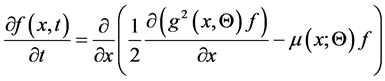


where S is the state space,  is the initial time and
  is the initial state of the pro- cess at time
 . Discrete Maximum Likelihood methods have been very popular in empirical work. The traditional DML uses an Euler-Maruyama algorithm with one step of duration:
 (26)
(26)
where .
.
Other methods use a Milstein approximation algorithm which, in most cases, give superior estimators compared to the Euler-Maruyama scheme. Our model specification for the fundamentals process states that

Letting , an Euler-Maruyama algorithm with one step of duration gives the discretization
 (27)
(27)
where  is a standard normal random variable.Hence, the approximated transitional PDF is assumed to be normal with mean
  and variance
 .
.
Now, take a sample  of N + 1 observations of the process f at time
 . The likelihood function of the sample observation
  is given by

where we define


The log-likelihood function is given by

The first order conditions entail
 (28)
(28)
 (29)
(29)
 (30)
(30)
 (31)
(31)
As indicated above, in our formulation, no approximation is necessary for estimation purposes given that a closed form solution for the likelihood function is available. We present the exact maximum likelihood estimation results as well as the pseudo maximum likelihood results below where we use velocity as economic fundamentals, as in [6] . This is slight departure from the monetary fundamentals specification based on the monetary model of exchange rate determination.
The estimates are presented below (Table 1).
It is clear that the model is consistent with the data.
4. The Target Zone Model
The target zone model considered here is driven by the behavior of the process governing the fundamentals process. We argued previously that a formulation of the series governing the fundamental determinant of exchange rate, f(t), is supposed to be guided by empirical considerations on the behavior of the series f(t) and therefore, models, whatever variables being considered as economic fundamentals, should not be agnostic about such behavior. In effect, the fundamental series f(t), as we have previously highlighted, depends on the model of exchange rate determination being considered. Again, the emphasis is put on the classical monetary model of exchange rate determination as in [18] .
As before, we assume that the dynamic behavior of the fundamentals is governed by the stochastic differential equation

where  and
and  are parameters to be estimated along with the other parameter of the model, which is
  in our model. As before, we use the fundamental equation for the exchange rate derived from the monetary model in continuous time

or equivalently,

where  is positive.
The model’s parameters are . These parameters need to be estimated simultaneously. Though the solution to the SDE governing the dynamic behavior of the fundamentals is not required for estimation purposes, it is necessary to find a closed form solution for the exchange rate, s(t), satisfying the fundamental equation. The solution is given in the following proposition.
Proposition 1. Suppose that the fundamentals, f(t), satisfy the stochastic differential equation

Table 1. Estimates of the parameters of the fundamentals process.
 (32)
(32)
Also, assume that the exchange rate is determined by the equation

Then a family of solutions for the exchange rate is given by
 (33)
(33)
where
 (34)
(34)
 (35)
(35)
where A and B are arbitrary constants.
Proof. The fundamentals are assumed to satisfy the SDE or GBM
 (36)
(36)
Guess that the exchange rate function is a time invariant function of the current fundamentals, that is, s(t) has the strong Markov property. Thus, we can set . By Ito’s lemma also known as Ito’s stochastic change of variable formula, we have
 (37)
(37)
Then we obtain
 (38)
(38)
This leads to the following second order differential equation given by
 (39)
(39)
This is a functional equation of the form
 (40)
(40)
This belongs to a well known class of ordinary differential equations known as the Cauchy-Euler or Equidimensional equation. Closed form solutions for such a class of differential equations exist. There are several methods for solving this class of ODEs. One such methods is he to use the theory of Laplace transforms. But, finding the inverse Laplace transform may be not that simple. The easiest solution method is to set  and obtain
 (41)
(41)
As usual, we solve the second order homogeneous ODE
 (42)
(42)
The characteristic equation is given by
 (43)
(43)
Given the definition of a, b, c, we have


Therefore, the general solution to the homogeneous equation is given by
 (44)
(44)
To find a particular solution, suppose it is given by .
.
Assuming that , it can be shown that the coefficients are given by


Finally, the general solution is given by
 (45)
(45)
Moreover, since , we have
 (46)
(46)
Since  and
and , we obtain then

where  and
and  are as defined above.
5. Monetary Interventions
The next task is to definitize the coefficients A and B. To do that, we consider different types of central bank interventions. As before, we consider a target zone . Introducing a target zone of this sort defines the fundamentals as a regulated Brownian motion. The point of the matter is that whenever the exchange rate falls within the band, the central bank or the monetary authorities do not intervene. Whenever the fundamentals touch one of the bands, the authorities do intervene. In the next section, we will consider the most widely used types of interventions we have previously examined such as Krugman’s infinitesimal marginal intervention [6] , Flood-Garber interventions [19] , and interventions in the sense of Bertola and Caballero [10] . Each type of interventions leads to different estimates of the integration coefficients A and B.
5.1. Krugman’s Type Interventions
As we have previously mentioned, Krugman infinitesimal marginal interventions assume that the monetary authorities intervene in the foreign exchange market so as to prevent the exchange rate from ever leaving the target zone band. At the time of interventions, . “Smooth-pasting” conditions imply that
 , and
, and . These two boundary conditions are sufficient to determine or definitize the constants of integration A and B. We have the following result which we will state as a corollary.
Corollary 2. Under Krugman interventions and with a geometric brownian motion for the fundamentals: , the exchange rate series, s(t), is given by
 (47)
(47)
where A and B are given by
 (48)
(48)
 (49)
(49)
 (50)
(50)
Furthermore, assuming symmetry, in the sense that  and
and , then we have
 (51)
(51)
 (52)
(52)
Proof. We have
 (53)
(53)
“Smooth-pasting” conditions imply
 (54)
(54)
 (55)
(55)
We obtain
 (56)
(56)
 (57)
(57)
For the symmetric case, we target zone becomes  so that the zone is symmetric about zero. We have
 (58)
(58)
A similar expression is obtained for B
 (59)
(59)
Also, in the symmetric case, we have
 (60)
(60)
 (61)
(61)
5.2. Flood-Garber Interventions
It is widely accepted in the literature that discrete interventions are more realistic than infinitesimal marginal interventions à la Krugman due to the fact that the central bank starts with a fixed amount of reserves which will eventually be exhausted [19] . In this section, we discuss the behavior of the exchange rate in the case of discrete interventions à la Flood-Garber. This type of intervention assumes perfect credibility of the zone from the point of view of market participants. We start by rewriting the exchange rate function as follows
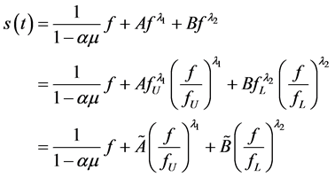
where  and
and . That is, we obtain
 (62)
(62)
The monetary authorities intervene in the foreign exchange market whenever f hits either the upper or lower bound of the target zone by placing the fundamental back in the middle of the band.
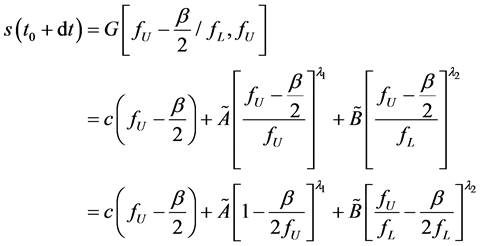
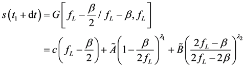
When the fundamentals hit the lower band  at time
 , we have
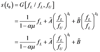 (63)
(63)
At time , market participants know with certainty that the monetary authori-
ties will reset f at the middle of the band, that is, at .
.
Hence,
 (64)
(64)
UIP implies no jumps and therefore

That is,

 (65)
(65)
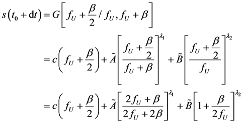
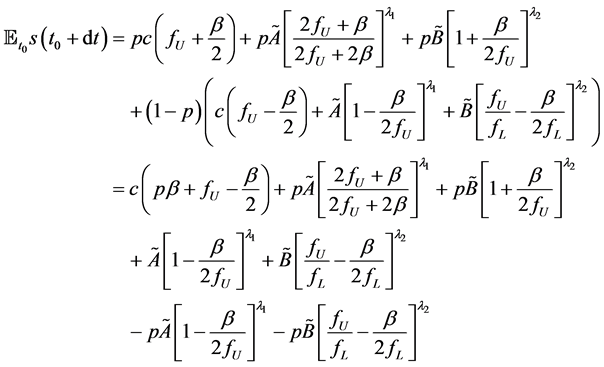
Similarly, at the instant  where the fundamentals hit the upper bound of the target zone,
we see that
 (66)
(66)
At the next instant , we have, as before
 (67)
(67)
That is,

Equivalently, we can write

We obtain the following system of linear equations
 (68)
(68)
 (69)
(69)
To solve the system, we set


The solution to the system is therefore obtained as
 (70)
(70)
 (71)
(71)
The complete solution to the model under Flood-Garber interventions can be summarized in the following proposition
Proposition 3. Under Flood-Garber interventions, the solution to the target zone model is given by

where


To complete the discussion under this type of interventions, we consider the symmetric case. This has only a theoretical value given that for our model, the fundamentals are either positive or negative.
Suppose that  and
and  so that the target zone is symmetric about zero. Then, it follows that
 ,
,  , and
, and . Also,


We present below a possible graph (Figure 1) for the exchange under some specific value of the target zone band.
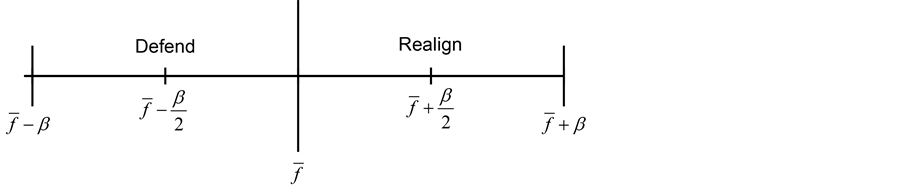
5.3. Bertola-Caballero Interventions
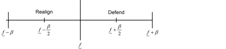
This type of intervention is justified by the fact that the monetary authorities start with a fixed amount of reserves which will eventually be exhausted and hence the target zone cannot be completely credible. Therefore, the assumption of perfect credibility is relaxed here. When the exchange rate hits either band limits, the monetary authorities either realign or mount a defense of the zone. Let p be the probability of realignment and 1 − p the probability that the monetary authorities mount a target zone defense. Suppose further that the fundamentals hit the upper bound, . At time
  when
when  is hit, we have
 (72)
(72)
At the next instant , we have
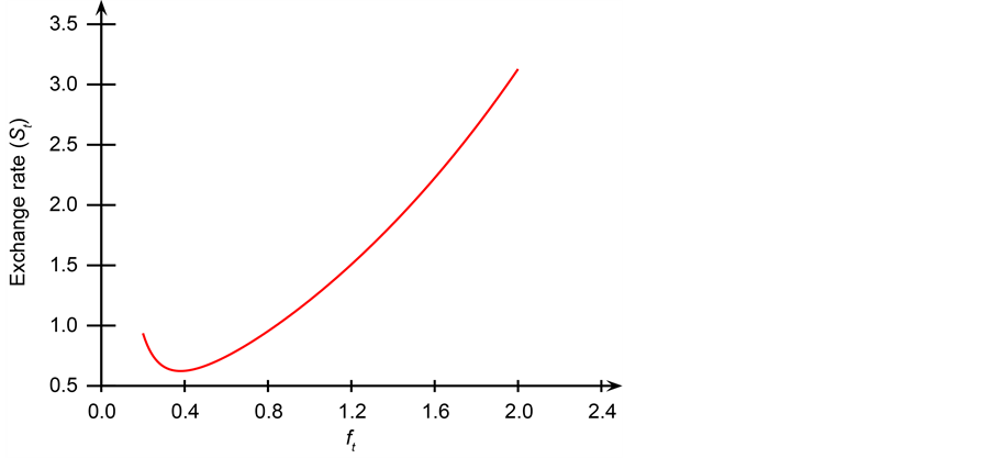
Figure 1. Relationship between f and s when f follows a GBM and Flood- Garber interventions.
1) With realignment (with probability p), we have a new band  and
and
2) If a defense is mounted, then the monetary authorities place the fundamentals back to the middle of the band:
Uncovered interest parity implies
 (73)
(73)
But, it is seen that
As before, UIP implies
 (74)
(74)
where


Now we consider the case where f hits the lower bound at time . Then
 (75)
(75)
If realignment occurs, then at time , we have a new band
 (76)
(76)
If a defense is mounted, then we obtain

This implies that

As before, UIP implies that exchange rate does not jump so that

We can rearrange this equation to obtain
 (77)
(77)
where


Finally, we consider the symmetric case. Suppose that ,
,  , so that the target band is symmetric about zero. Then, we have
 (78)
(78)
 (79)
(79)
 (80)
(80)
 (81)
(81)
These results are summarized in the following proposition.
Proposition 4. Under Flood-Garber interventions, the solution to the target zone model is given by

where
 (82)
(82)
 (83)
(83)
and as given above
 (84)
(84)
 (85)
(85)
 (86)
(86)


and  and
and  are as before.
Table 2. SMM estimates of the Flood-Garber target zone model for Japan.
6. Estimation Results of the Model’s Parameters
In this section, we present some estimates of the model’s parameters for the Krugman’s and Flood-Garber’s types of interventions. We use Daily exchange rate data for Japan and Sweden from 1987 to 1990. Though the data are relatively old, we use it to illustrate the findings that the model gives some satisfactory results contrary the basic target zones models in the literature. The estimation technique being used is the Simulated Method of Moments (SMM) procedure [17] . Our task here is to estimate the parameters ,
,  ,
,  ,
,  and
and  of the model. We obtain the following estimates for Japan data (Table 2).
As indicated by the table, the estimates are quite reasonable in magnitude and, as expected, have the correct signs. Moreover, the J-Statistic of the one overidentifying restriction is not rejected and therefore the model does a good job in fitting the data, at the most commonly used significance levels.
We also found that the model does not perform well in the case for the Krugman marginal interventions. The estimates are reasonable in signs and magnitudes. However, the high value of the J-Statistics indicates that the model is not supported by the data. In essence, this can be due to the fact that it is commonly not easy to estimate these models efficiently.
7. Conclusion
In this paper, we have derived analytical or closed form expressions for the exchange rate function under the assumption that the fundamentals follow a geometric Brownian motion within the target zone band. Preliminary estimates from Simulated Method of Moments (SMM) show that the data do not show great support for the Krugman infinitesimal marginal interventions in the foreign exchange market, as indicated by the high value of the J-statistic. However, we found strong evidence for the target zone model for Flood-Garber interventions for the case of Japan, as indicated by the low value of the J-statistic. This indicates that it is likely that Japan has used an unofficial exchange rate target zone band during the 1987-1990 period. This is not a surprise due to the fact that central banks do not often reveal their intervention strategies. No such evidence has been found for the case of Germany.
Cite this paper
Cupidon, J.R. and Hyppolite, J. (2016) A Target Zone Model Where the Fundamentals Follow a Geometric Brownian Motion. Journal of Mathematical Finance, 6, 866-886. http://dx.doi.org/10.4236/jmf.2016.65058
References
- 1. Mark, N.C. (2001) International Macroeconomics and Finance: Theory and Econometric Methods. Wiley-Blackwell.
- 2. De Jong, F. (1994) A Univariate Analysis of EMS Exchange Rate Using a Target Zone Model. Journal of Applied Econometrics, 9, 31-45.
http://dx.doi.org/10.1002/jae.3950090104 - 3. Svensson, L.E.O. (1992) An Interpretation of Recent Research on Exchange Rate Target Zones. Journal of Economic Perspectives, 6, 119-144.
http://dx.doi.org/10.1257/jep.6.4.119 - 4. Chung, C.-S. and Tauchen, G. (2001) Testing Target Zone Models Using Efficient Methods of Moments. Journal of Business and Economic Statistics, 19, 255-277.
http://dx.doi.org/10.1198/073500101681019891 - 5. Spencer, M. and Smith, G.W. (1992) Estimation and Testing in Models of Exchange-Rate Target Zones and Process Switching. In: Krugman, P. and Miller, M., Eds., Exchange Rate Targets and Currency Bands, Cambridge University Press/CEPR, 211-239.
- 6. Krugman, P.R. (1991) Target Zones and Exchange Rate Dynamics. The Quarterly Journal of Economics, 106, 669-682.
http://dx.doi.org/10.2307/2937922 - 7. Svensson, L.E.O. (1991) The Simplest Test of Target Zone Credibility. IMF Staff Papers.
- 8. Weber, A.A. (1991) Reputation and Credibility in the European Monetary System. Economic Policy, 6, 57-102.
http://dx.doi.org/10.2307/1344449 - 9. Bertola, G. and Svensson, L.E.O. (1992) Stochastic Devaluation Risk and the Empirical Fit of Target Zone Models. Review of Economic Studies, 60, 689-712.
- 10. Bertola, G. and Caballero, R.J. (1992) Target Zones and Realignments. American Economic Review, 82, 520-536.
- 11. Belessakos, E. and Loufir, R. (1993) Exchange Rate Target Zones in a Utility Maximizing Framework. Annales D’economies et de Statistique, No. 31, 33-50.
- 12. Jorion, P. (1988) On Jump Processes in the Foreign Exchange and Stock Markets. The Review of Financial Studies, 1, 427-445.
http://dx.doi.org/10.1093/rfs/1.4.427 - 13. MacDonald, R. and Taylor, M.P. (1993) The Monetary Approach to the Exchange Rate: Rational Expectations, Long-Run Equilibrium, and Forecasting. International Monetary Fund Staff Papers.
- 14. Mark, N.C. and Sul, D. (2001) Nominal Exchange Rates and Monetary Fundamentals: Evidence from a Small Post-Bretton Woods Panel. Journal of International Economics, 53, 29-52.
http://dx.doi.org/10.1016/S0022-1996(00)00052-0 - 15. Meese, R. and Rogoff, K. (1983) Empirical Exchange Rate Models of the 1970s: Do They Fit out of Sample? Journal of International Economics, 14, 3-24.
- 16. Dornbusch, R. (1976) Expectations and Exchange Rate Dynamics. Journal of Political Economy, 84, 1161-1176.
http://dx.doi.org/10.1086/260506 - 17. Hansen, L.P. and Scheinkman, J.A. (1995) Back to the Future: Generating Moment Implications for Continuous-Time Markov Processes. Econometrica, 63, 767-804.
http://dx.doi.org/10.2307/2171800 - 18. Taylor, M.P. and Sarno, L. (1998) The Behavior of Real Exchange Rates during the Post-Bretton Woods Period. Journal of International Economics, 46, 281-312.
http://dx.doi.org/10.1016/S0022-1996(97)00054-8 - 19. Flood, R. and Garber, P. (1984) Collapsing Exchange Rate Regimes: Some Linear Examples. Journal of International Economics, 17, 1-13.
http://dx.doi.org/10.1016/0022-1996(84)90002-3