Journal of Mathematical Finance
Vol.3 No.4(2013), Article ID:40096,15 pages DOI:10.4236/jmf.2013.34051
A Mathematical Approach to a Stocks Portfolio Selection: The Case of Uganda Securities Exchange (USE)
1Department of Investments and Research, STANLIB, Kampala, Uganda
2Division of Actuarial Sciences, University of Cape Town, Rondebosch, South Africa
3Department of Mathematics, College of Natural and Applied Sciences, University of Dar es Salaam, Dar es Salaam, Tanzania
Email: fredrickmay@gmail.com, mayanjaf@stanlib.com, sure.mataramvura@uct.ac.za, mahera@math.udsm.ac.tz
Copyright © 2013 Fredrick Mayanja et al. This is an open access article distributed under the Creative Commons Attribution License, which permits unrestricted use, distribution, and reproduction in any medium, provided the original work is properly cited.
Received August 23, 2013; revised October 23, 2013; accepted November 6, 2013
Keywords: Portfolio Optimisation; Uganda Securities Exchange (USE); Stocks; Modern Portfolio Theory (MPT); Markowitz; Portfolio Diversification; Frontier; Efficient Frontier; Constraints
ABSTRACT
In this paper, we present the problem of portfolio optimization under investment. This area of investment is traced with works of Professor Markowitz way back in 1952. First, we determine the probability distribution of the Uganda Securities Exchange (USE) stocks returns. Secondly, we develop unrestricted portfolio optimization model based on the classical Modern Portfolio Optimization (MPT) model, and then we incorporate certain restrictions typical of the USE trading or investment environment and hence, develop the modified restricted model. Thirdly, we explore the possibility of diversification under a portfolio of averagely correlated assets. Determination of the model parameters and model development is all done using Excel spreadsheets. We explicitly go through the mathematics of the solution methods for both models. Validation of the models is done using the USE stocks daily trading data, in which case we use a random sample of 6 stocks out of the 13 stocks listed at the USE. To start with, we prove that USE stocks log returns are normally distributed. Data analysis results and the frontier curves show that our modified (restricted) model is valid as the solutions are all consistent with the theoretical foundations of the classical MPT-model but inferior to the unrestricted model. To make the model more useful, accurate and easy to apply and robust, we programme the model using Visual Basic for Applications (VBA). We therefore recommend that before applying investment models such as the MPT, model modifications must be made so as to adapt them to particular investment environments. Moreover, to make them useful so as to serve the intended purpose, the models should be programmed so as to make implementation less cumbersome.
1. Introduction
Portfolio Optimization also commonly referred to as Portfolio selection is the problem of allocating capital over a number of available assets in order to maximize the “return” on the investment while minimizing the “risk” [1]. Research into the development of models for portfolio selection under uncertainty dates back to the fifties with Markowitz’s (1959) pioneering work on meanvariance efficient (MV) portfolios [2].
Although the benefits of diversification in reducing risk have been appreciated since the inception of financial markets, the first mathematical model for portfolio selection was formulated by Markowitz [3,4]. In the Markowitz portfolio selection model, the “return” on a portfolio is measured by the expected value of the random portfolio return, and the associated “risk” is quantified by the variance of the portfolio return. Markowitz showed that, given either an upper bound on the risk that the investor is willing to take or a lower bound on the return the investor is willing to accept, the optimal portfolio can be obtained by solving a convex quadratic programming problem. This mean-variance model has had a profound impact on the economic modeling of financial markets and the pricing of assets: The Capital Asset Pricing Model (CAPM) developed primarily by [5,6] was an immediate logical consequence of the Markowitz theory. Work on models for portfolio optimization continued, with much of it concentrated on improving the mean-variance (Modern Portfolio Theory) model. Developments in portfolio optimization are stimulated by two basic requirements: 1) adequate modeling of utility functions, risks, and constraints; 2) efficiency, i.e., ability to handle large numbers of instruments and scenarios [7]. All models directly or indirectly emerged from the Modern Portfolio Theory model, as most research tried to make the assumptions more realistic to real life; some have incorporated transaction costs in the model [8]. Others proposed alternative ways of measuring risk as opposed to use standard deviation of the stock returns. Many practitioners were not fully convinced of the validity of the standard deviation as a measure of risk [9]. They are certainly unhappy to have small or negative profit, but they usually feel happy to have larger profit. This means that the investors’ perception against risk is not symmetric around the mean [10]. Unfortunately, however, some studies of stock prices in Tokyo Stock Market [11] revealed that most of asset returns are not normally nor even symmetrically distributed.
Also, much has been done in developing algorithms for portfolio optimization using various approaches. This is because to carry out portfolio optimization one needs some form of software, which must have in built algorithms. There are software companies dedicated to developing software for portfolio optimization, and these software are either spreadsheets applications and/programs. Most commonly used software is Solver or Optimizers; these are software tools that help users to find the “best” way to allocate resources. To carry out portfolio optimization there must be portfolios in existence, such that one seeks only to find the optimal set of weights for this portfolio. These portfolios are investment portfolios held and traded in Stock (Securities) Exchanges. Stock exchanges are markets where government and industry can raise long-term capital and investors can buy and sell securities [12]. It is an organized market where buyers and sellers of securities meet as dealers/brokers represent them and acquire or sell securities. The Uganda Securities Exchange (USE) is one such market; it was established in 1998 as a result of a Government Policy of transforming the economy of the country from a public sector to the private sector basis [13].
The USE represents a vital link between companies with capital needs and the public with savings to invest. The Uganda Clays was the first company to be listed in 1999, and by 2004 there were 5 companies trading. Today USE has 13 companies listed and trading in the various securities available [14]. Securities that are currently traded at the Exchange include Government Bonds, Corporate Bonds and Ordinary Shares. There are a number of individual investors, financial institutions and companies that currently hold investment portfolios among these listed companies at USE. These investors, financial institutions and companies use brokers and investment managers to trade and manage their portfolios. These investment managers or brokers use the qualitative analysis approach of market surveillance intelligence and speculation. This is mainly because the models available for optimization of portfolios have not been customized to the Uganda Securities Market and cannot be applied in the market. The need to adapt the models arises from the fact that different assets behave differently in different investment environment [10]. However, the Uganda Securities Market has developed over time and is still growing as more companies become listed at the USE; this has made the market analysis more complex. Therefore, there is need for a mathematical approach of using optimization models to analyze and manage the investment portfolios so as to complement the conservative methods currently used. To appreciate the importance of adaptation rather than adoption of investment models to various trading environments, let us briefly list down some of the characteristics of one of the developed securities exchanges-the New York Securities Exchange (NYSE) so as to have a clear comparison with the USE: The NYSE was started way back in 1792, with its first constitution adopted in 1817. NYSE is the world's largest cash equities market. It is the world's largest stock exchange by market capitalization of its listed companies at US  trillion, with an average trading value of approximately US
 billion, as of August, 2008. It provides a means for buyers and sellers to trade shares of stock in companies registered for public trading. It opens for trading Monday - Friday between 9:30 am - 4:00 pm. All NYSE stocks can be traded via its electronic Hybrid Market, and customers do send orders for immediate electronic execution. In 2007, NYSE joined a merger with some other stock exchanges to form; NYSE Euronext, and as of March, 31, 2011, NYSE Euronext has approximately 7950 listed issues, a total global market capitalization of US
 trillion and it’s equity exchanges transact an average daily trading value of approximately US
  billion
  Clearly, when we compare the two securities exchanges it would be wrong to assume that since a model is applicable to the NYSE then, it will also be applicable to the USE without any changes. And therefore this justifies the focus of our study on examining and testing the applicability of the classical mean—variance model to the USE.
2. Testing Whether Log Returns Are Normally Distributed
Six Stocks namely, British American Tobacco Uganda (BATU), Bank Of Baroda Uganda (BOBU), Development Finance Company of Uganda (DFCU), Stanbic Bank Uganda (SBU), East African Breweries Limited (EABL) and Uganda Clays Limited (UCL) were randomly selected from the 13 stocks available at the USE. Their daily trading data was down-loaded from the USE website; www.use.org as per the  The data we down-loaded was for four years
 , The spreadsheets used were the excel
  spreadsheets, this is where the stocks returns were calculated using the data. When calculating the stocks returns we used the formula;

we determined the frequencies of the log returns using the “FREQUENCY” excel in built function. Using these frequencies we calculated the cumulative frequencies using the formula;
And, this gave us the actual stocks ’s for the historical data. Then we simulated the cumulative frequencies for a normally distributed data set with the same mean and standard deviation as each of our stocks. Here we used the excel’s “NORMDIST” function which produces cumulative frequencies that are normally distributed given the mean and standard deviation of any data set. We then plotted the actual cumulative frequencies of the historical data and the simulated normal distribution frequencies on the same graph, for each stock. The resulting graphs are as shown in figures 1-4.
From the graphs, as analyzed for each stock we see that there are some small deviations from normal distribution for the actual data but, the deviations are not significant enough for us to reject normal distribution of the log returns. These slight deviations could be because of skewness and kurtosis. However, to avoid making wrong conclusions about the distribution of our log returns we took a step further the deviations at the extreme ends are due to outliers. To accomplish this task we plotted the stocks log returns for each stock as shown in figures 5-8.
From the results we note that these stocks have some two to three “extreme months”. That is, for each stock there is a month or two where the monthly log returns are either extremely high or extremely low as compared to the average monthly returns, and this adequately explains the slight deviations between the cumulative curves. Since for real data outliers are certainly expected, we therefore comfortably concluded that the log returns of the stocks at USE are normally distributed, which confirms to the general findings that log returns are normally distributed, [15,16]. Note that instead of analyzing the stocks log returns by plotting them, we could have used the method of calculating the kurtosis and skewness parameter values to determine whether they lie within the theoretical normal distribution values. But, this method was not preferred because the kurtosis and skewness values are not conclusive since they are highly dependent on the data size. In fact for the same data set, selecting different sample sizes results in to totally different parameter values for both kurtosis and skewness, [17].
3. Model Parameters and Model Development
the correlation of the stocks and hence correlation matrix was determined using the excel’s function “CORREL” for determining the correlation, this function uses the formula;
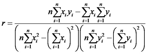
For more details about the setup of the model parameters in the excel spreadsheet and explicit results you may refer to page 45 of [1]. Note that this formula is based on a sample of historical returns of any two assets, this means that the formula provides sample correlation coefficient (r) of the two assets rather than the population or “true” correlation coefficient , That is, it might not be a true representation of the “true” correlation coefficient. Despite the problems of using a sample of historical returns to estimate the correlation coefficient between two assets [18]. It remains a very popular technique among investors and investment analysts because the formula for this approach has already been programmed in most calculators and spreadsheet programs. However care has to be taken when interpreting the meaning of sample correlation coefficient:
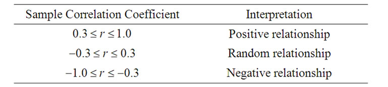
Referring to our correlation matrix on page 45 [1], our sample correlation coefficient is ;
; 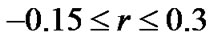 which according to the interpretation by [18] means that our stocks returns have a random relationship. It is therefore for this very reason that we did not use Markowitz's principle of adding negatively correlated assets to the portfolio to improve it through diversification, simply because not any one of our portfolio stocks have a strong negative correlation. So we formulated a condition for an additional stock to improve the frontier of the portfolio as we shall show in the next section. For now we try to formulate and solve the MPT-model using USE data.
4. Mathematical Formulation of the Model
Recall that the MPT model is a theory of investment which tries to minimize risk (standard deviation of the returns) for a given level of expected return, by carefully
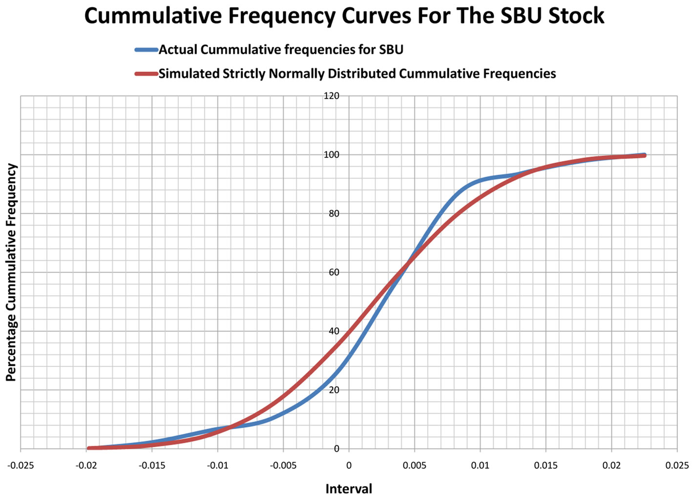
Figure 1. SBU stock.
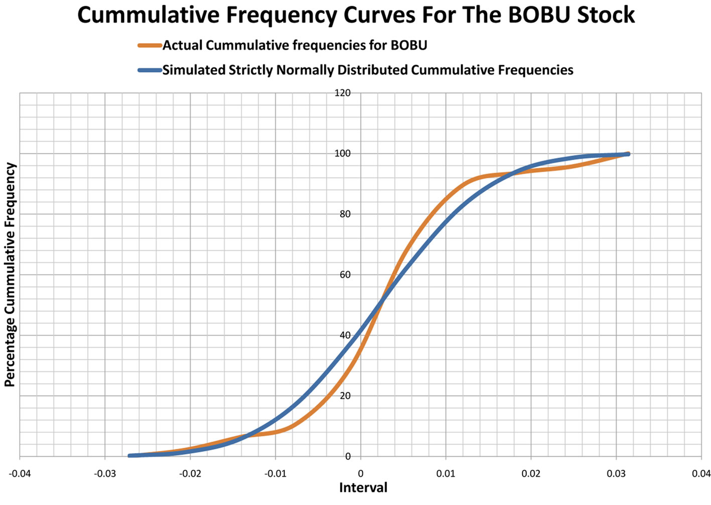
Figure 2. BOBU stock.
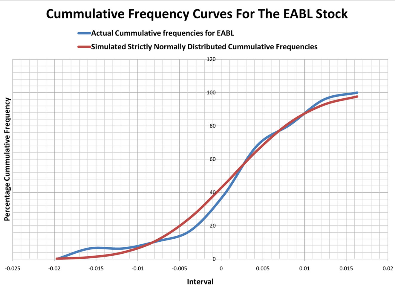
Figure 3. EABL stock.
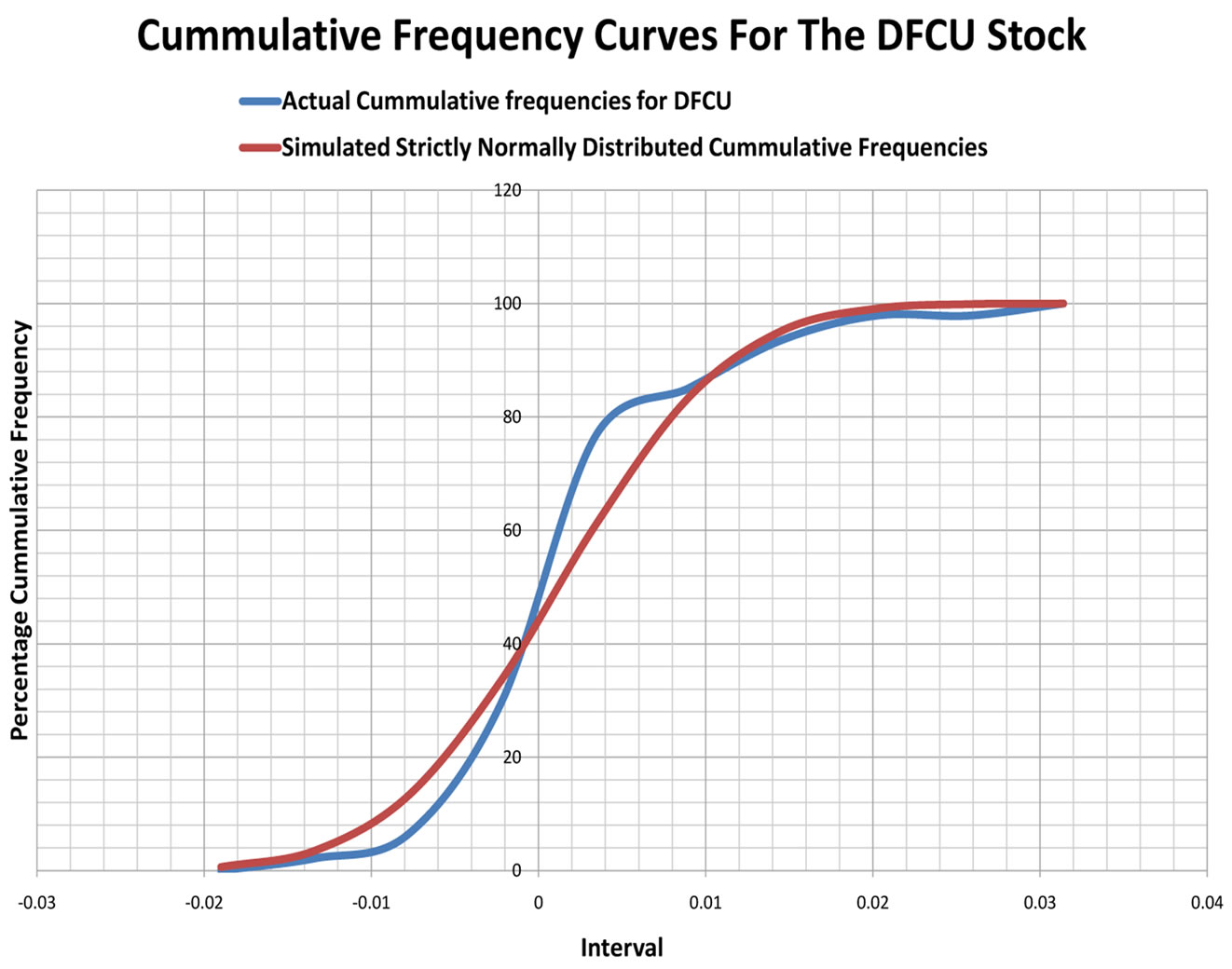
Figure 4. DFCU stock.
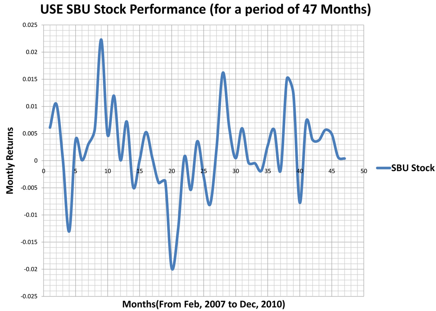
Figure 5. SBU stock performance.
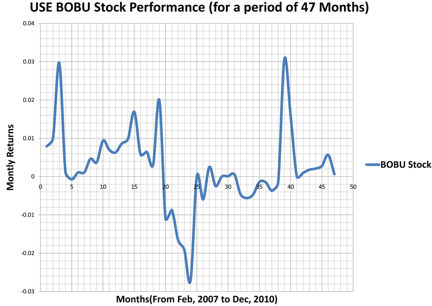
Figure 6. BOBU stock performance.
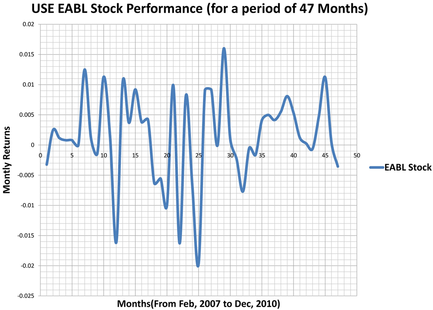
Figure 7. EABl stock performance.
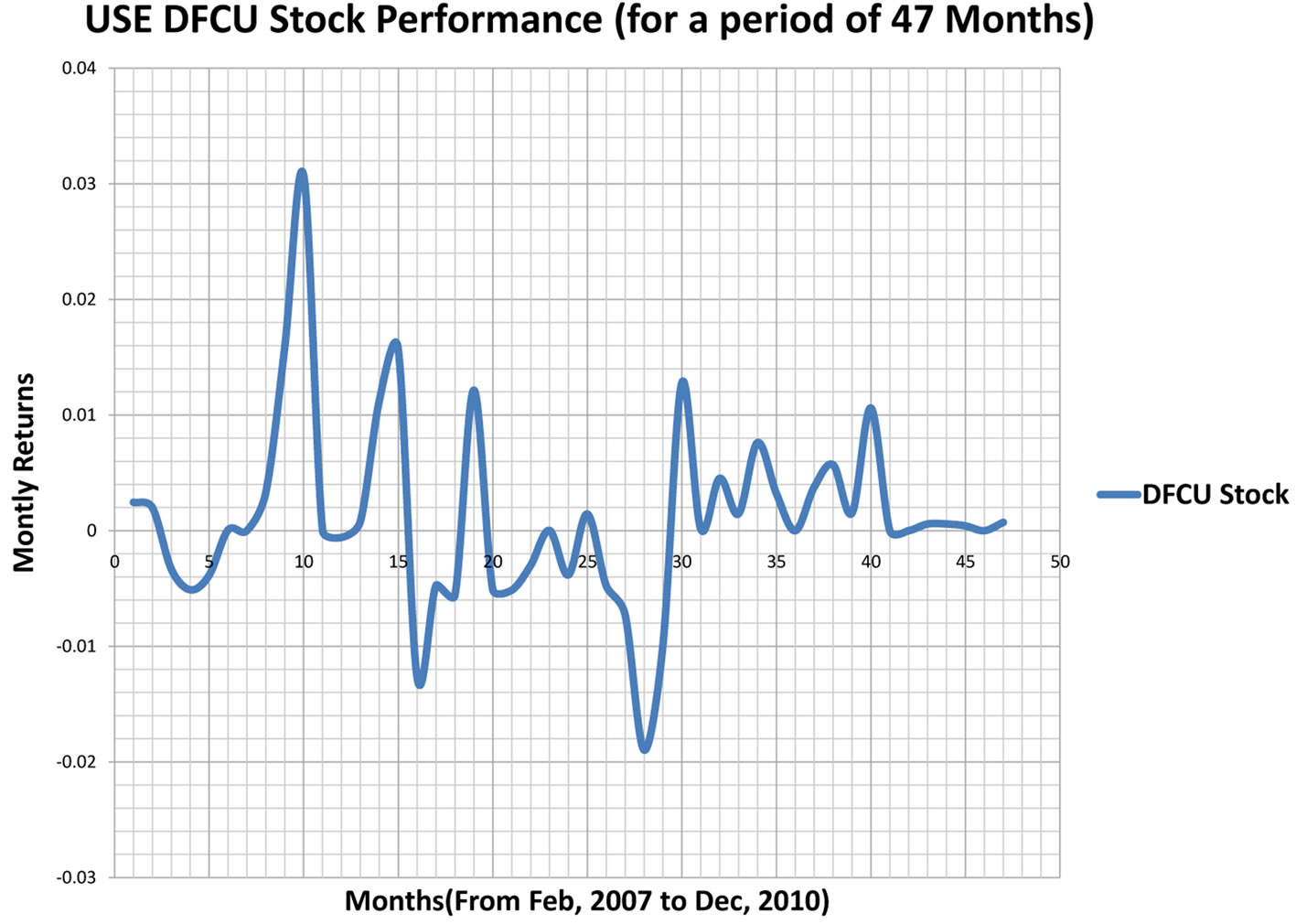
Figure 8. DFCU stock performance.
choosing the proportions (weights) of various assets available. Therefore the model can be written as:
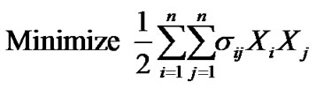

That is, given the target expected rate of return of the portfolio , find the portfolio strategy that minimizes the portfolio variance in returns
 .
.
5. The Solution Method for the n-Asset Model
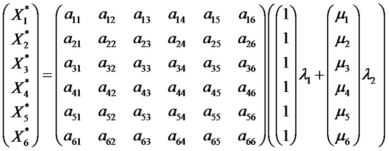
First, we note that it is more convenient and easier to use vector and matrix notation, so we formulate this model in matrix notation;
 (5.1)
(5.1)
where , is column vector of portfolio weights for each security.
 is the covariance matrix of the returns.
 is the desired level of expected return for the portfolio.
Note that in this model formulation;
1) The admissible set includes short selling, i.e. portfolio positions with negative weights 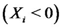 are allowed.
2) The parameter  is exogenously given.
3) The model (5.1) is a convex quadratic programming problem (i.e., the objective function is quadratic, with linear constraints and the feasibility set S is convex).
4) The solution(s) of the program depend(s) on the parameter .
.
To avoid degeneracies we impose the following technical conditions:  All first and second moments of the random variables exist.
 The vectors
  are linearly independent. That is, no two securities can have the same expected return
 . We note that this is typically the case when using real data.
 The covariance matrix is strictly positive definite. The positivity of the covariance matrix means that all the
 ![]() assets are indeed risky, and this is the case of our portfolio since we considering stocks only.
assets are indeed risky, and this is the case of our portfolio since we considering stocks only.
To illustrate why we require  to be strictly positive definite, suppose;
Then there exists a portfolio whose return  has zero variance. This implies that
 , essentially, that this portfolio is risk less. But, this contradicts the idea that our portfolio consists of only risky assets. At this stage, before we attempt to solve our formulated problem there is need to see whether the problem has been well formulated. That is whether a unique solution exists.
proposition 1.
Model problem (5.1) is a convex quadratic problem with a unique convex solution.
proof.
The function  defines a quadratic form. The matrix
  is symmetric and positive definite (from condition
![]() ), this means that
), this means that  is strictly convex. The constraints are linear, which guarantees that
 ![]() is a convex solution space. Moreover condition
is a convex solution space. Moreover condition  implies that the gradients of the constraints are linearly independent, which guarantees a unique solution. Therefore, if conditions
  hold, the model problem (5.1) has a unique solution and hence well formulated.
6. Solution to the Formulated Model
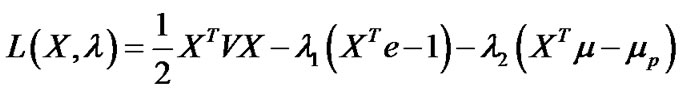
We therefore can proceed to determine the solution, first we note that model problem (5.1) is a constrained classical optimization problem, with equality constraints. It can therefore be solved by the Lagrangian method. The Lagrangean function1 for the model is
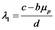
If conditions  hold, the solution to the above problem is2;
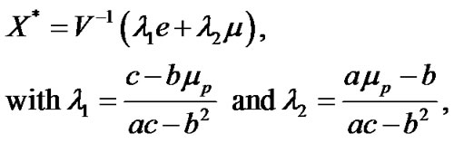 (6.1)
(6.1)
where
Note that  and
and  depend on
 , which is the target portfolio mean prescribed in the variance minimization problem. The variables
  can be determined since
  and
and  are known.
Hence

can be solved. where
is the optimal portfolio weights. For , Equation (6.1) becomes;
The variance3  for the optimal portfolio
  is given by
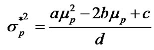 .
.
The resulting frontiers of the un constrained problem above for the Lagrange method is as shown in figure 9 with the global minimum variance portfolio marked red on the frontier4.
However this is ideal as there are restrictions in the USE market for example no short selling, and there is a specified sum to be invested in a particular stock therefore we incorporate restrictions
7. Effect of Incorporating Restrictions to the Model
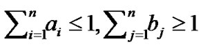
Imposing the restriction;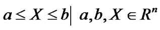 , where in general we assume that
hold.
Note that  is necessary for the portfolio optimization problem to have a solution and
  assures us that total wealth available will be invested.
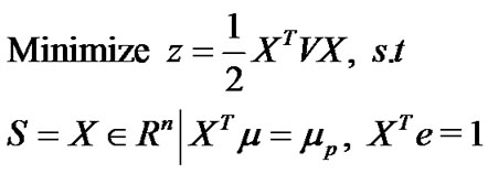
Our optimization problem (5.1) would therefore be:

To be specific we require that the weights are nonnegative,  therefore, we shall restrict
 , So we have
 . Our problem therefore is:
 (7.1)
(7.1)
Next, we now seek to write our model as a quadratic programming problem. First we recall that a quadratic programming problem has the general form:

The function  defines a quadratic form, the matrix
  is symmetric and positive, the constraints are linear which guarantees a convex solution space. The solution to this problem is based on the Karush-KuhnTucker (KKT) conditions5. Applying the KKT conditions to the model problem above for we which we seek a solution becomes6;
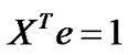
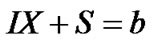
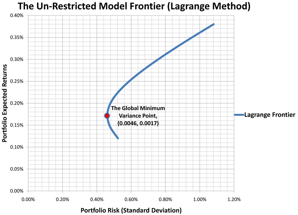
Figure 9. The unconstrained frontier (lagrange method).
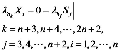
And according to the  theorem we must consider at most
  different cases to find the optimal solution. It is therefore very evident at this stage, what impact the weight restrictions have had on the solution procedure. This system unlike the unrestricted model we had before, cannot be solved analytically for
  assets. Therefore we have to seek numerical algorithms to determine the optimal solution. However, the good news is that with the current computer advancements we do not have to struggle with the algorithms. Powerful algorithms for numerical methods have been developed in various softwares. For this particular problem we shall use the excel solver
 , which uses the Newton Raphson algorithm to find the optimal solutions numerically. These optimal portfolio returns were plotted against the optimal standard deviation and the resulting frontier is as shown in figure 10.
In an attempt to make a comparative analysis of the effect of restriction on the level of returns we plotted both frontiers on the same graph as shown in figure 11.
From the graph notice that the unconstrained frontier is superior to the constrained frontier. That is, for every risk level, the unconstrained frontier gives a higher or equal return as compared to the constrained frontier. Which is as expected, since constraints or restrictions on investment have a negative affect on the level of returns. This is in line with the theoretical findings [20].
8. Diversification under a Portfolio with Averagely Correlated Assets
In consideration of diversification constraint 4., we try to explore Mathematically the effect of increasing or reducing the number of stocks held in a portfolio on the frontier. That is, we shall examine the necessary and sufficient conditions for a security to improve the Markowitz hyperbola (frontier).
Let  be a set of
 ![]() securities among which we may choose for our portfolio. Additionally, let
securities among which we may choose for our portfolio. Additionally, let
 .
.
Also, let  and
and  be the Markowitz hyperbolas for security sets
  and
and  respectively.
proposition 3.
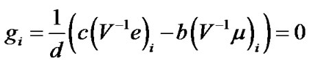
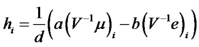
Unique portfolio weights can be determined for securities that lie on the hyperbola as a linear function of the portfolio expected return, . That is,
  , where g and h are known constants for a particular portfolio.
proof.
Recall that we have
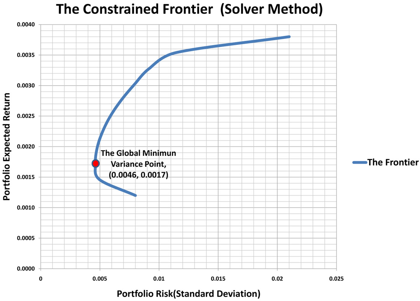
Figure 10. The constrained frontier.
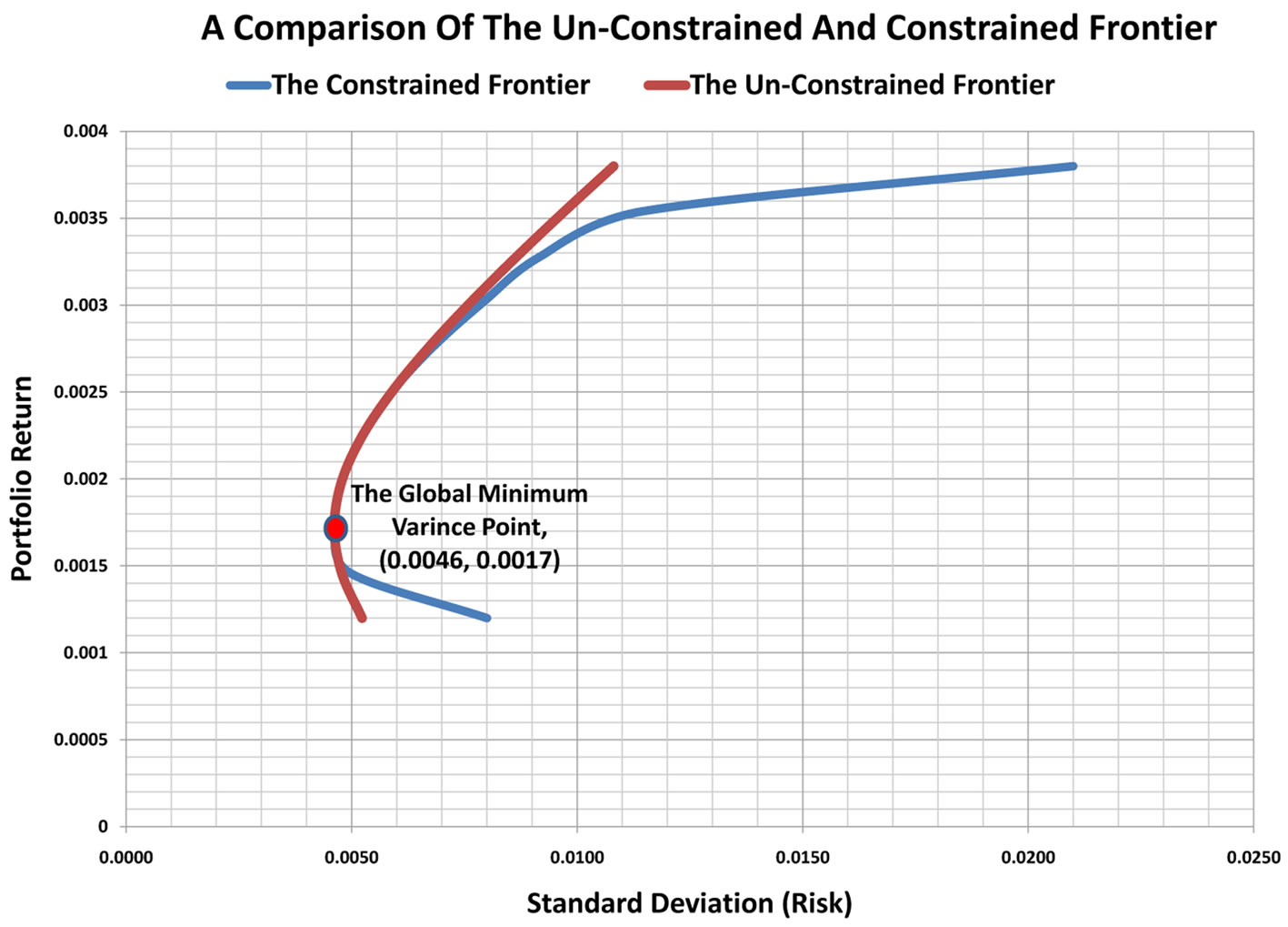
Figure 11. The unconstrained and constrained frontiers.
for the un-restricted model problem. Where;
 , and
, and 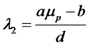
Substituting for  gives;
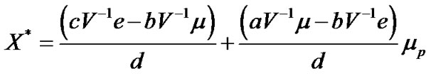
Therefore,
 (8.1)
(8.1)
Theorem 8.1 Consider the above equation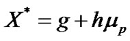 , then;
1) If , then
 .
.
2) If  and
and , then
  and any point on
  has a non-zero fixed weight of the
  security.
3) If , then
 , so
, so  and
and  are tangent at exactly one point.
proof of (i).
Assume . Then
 .
.
Hence, the  security has a zero weight for every point on
 , and so it may be disregarded from portfolio consideration as it does not improve the hyperbola. But, upon removing the
  security from
 , we are left with
 . That is, the set of securities that optimize
 . Therefore,
 .
.
proof of (ii).
If  and
and , the expression
  equals
  and thus, any point on
  has a fixed non-zero weight of the
  security. Recall that points on
  have unique portfolios associated with them (refer to Proposition
 ) and that each point on
  has a non-zero weight of the
  security, we conclude that
 .
.
proof of (iii).
If , the linear function
  will have exactly one root at
 .
.
Therefore,

will be the only  such that
if ; that is,
  will be the only value of
  at which the Markowitz hyperbolas
  and
and  intersect. That is because
 ,
, .
.
Therefore,  , so the
  security is not involved.
But,  and
and  cannot cross each other so
  is inside or on
 . Therefore, the intersection of the two Markowitz hyperbolas must be a tangent point. Also, since
  and
and  only intersect at one point, it is clear that
 .
.
corollary 1.
 .
.
proof.
Suppose  does not hold. That is,
  and
and , or
, or , (in part
 is not conditioned because if
  whether
  or
or  the effect of the
  security carries the same Mathematical implication on
 ).
).
From , if
, if  and
and , then
  which contradicts
 . Also, from
  if
if , then
  which contradicts
 . Therefore, we conclude that
  implies
 . But, from
 , if
, if , then
 . Hence,
 .
.
Theorem 8.2
![]()
proof.
Assume , then from Equation (8.1) we have;
![]()
From
![]()
we have:
 (8.2)
(8.2)
and from
![]()
we have:
 (8.3)
(8.3)
Combining Equations (8.2) and (8.3) we get;
 (8.4)
(8.4)
In Equation (8.4) above we see that if![]() , then we conclude
, then we conclude
 which implies
 , and that
 , which is impossible!(refer to the proof of
 , where we proved that
 ). So
). So![]() .
.
Since![]() , but
, but ![]() which implies that also,
which implies that also,![]() . But
. But  therefore,
![]() . Hence
. Hence
![]() .
.
converselyAssume
![]() .
.
Then clearly
 .
.
But recall
 . So,
. So, .
.
Also,
 .
.
But recall
 . So,
. So, .
.
Thus,
![]()
which implies .
.
corollary 2
![]()
Proof.
From corollary 1 have;  if
if . Also, from theorem
  we have;
![]() .
.
Therefore, corollary 1 and Theorem  together imply;
![]() .
.
And, corollary 2 s the final result that we have been seeking to prove. corollary 2 provides a necessary and sufficient condition for some security,  , to improve a Markowitz hyperbola.
This will be so provided the addition of the  to the existing security set (portfolio)
  is such that the new covariance matrix
 , which includes
 , is invertible and the condition;
![]()
does not hold. If one wonders how this is so; when
![]()
does not hold, corollary 2 implies that then . But, from proof of
  we saw that when
 , these two have only one tangent point and therefore one of the two hyperbolas is greater than the other. And in this case it is the hyperbola of the portfolio to which an extra security has been added that is greater than the original one.
However, since the stocks in our portfolio have a random relationship, we preferred to use the condition we proved in corollary 2 of chapter , which is independent of the correlation of the assets; the condition only required us to compute the new covariance matrix
 , that includes the additional stock and then check if
does not hold, if and when this condition does not hold then the new stock added will improve the frontier. We started with a portfolio of three stocks namely; DFCU, BOBU and SBU with covariance matrix , then we added a new stock UCL and computed the new covariance matrix
  and
and , checked the condition and found that;
 we further added a fifth stock EABL and again computed the new covariance matrix
  and
and  which included the new EABL stock, we got
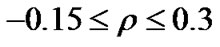
and upon plotting the three frontiers together on the same graph, we observed that the frontier for the portfolio of  stocks was above that of the
  stocks which in turn was above that of
  stocks, as shown in figure 12.
Therefore our condition for diversification as derived in in chapter , corollary 2 is valid and applicable for the USE (restricted) model. Hence, an investor can still reduce portfolio risk even when his/her portfolio is made up of stocks only. Therefore, even for investors who are less risk averse, it is still possible for them to reduce portfolio risk by increasing the number of stock in a portfolio.
9. Conclusions
In this study, we have identified that the USE stock market as a whole is stochastic, as there are no particular months where all stocks returns are low or high, and each stock behaves randomly. This is seen from the graphs showing individual stocks performance—figures 5-8, in which case we concluded that the stocks have a random relationship as their over all correlation coefficient ;
; 
We have also noted that the "BATU" stock is the most volatile stock among them all but, still the most profitable among a sample of the 6 stocks.
We have proved that the log returns of the USE stocks are normally distributed, which implies that their returns have a log normal distribution.
We have also discussed in detail the Mathematics and theoretical advancements behind the classical MPT-model and tested these arguments against the USE stocks data for which we have found out that the data analysis results agree with the theory. First, we have showed that the plot of stocks returns against their standard deviation (risk) is a hyperbola for both the unrestricted and the restricted optimization model problem. Secondly, we have also noted that increasing the number of stocks in the portfolio improves the frontier, which is in agreement with the MPT-model theory. However, since our portfolio assets had a random relationship we could not rely on Markowitz’s idea. So we have provided a condition that each extra additional stock should satisfy so as to improve the frontier. In other words, it is not necessarily true that every additional stock improves a frontier. It will only do so as long as corollary 2 condition is satisfied.
Finally, we found out that the solution of the unrestricted model problem is superior (for every level of risk, the unrestricted frontier gives an equal or higher level of returns as compared to the restricted frontier of the same portfolio) to that of the restricted model problem, this as seen from Figure 11, in which the two frontiers were plotted together.
Though the Mathematics involved is tedious and at times complex in general, the users of these models do not need to worry because with the current computer advancements a number of softwares have been developed ready to use with out bothering about the Mathematics.
Figure 12. Diversification based on corollary 2.
10. Recommendations
We recommend the use of computer programmes as they help to enhance the performance of the optimization software and also automate the various calculations that would other wise be performed manually in spreadsheets. We also, recommend financial institutions and any other investors who use investment models to always examine, test and adapt these models to their investment environment before applying or using them to make investment decisions, since most of these models have underlying assumptions which have diverse implications mathematically, financially and economically for different investment environment.
In the study of the effect of imposing certain restrictions we focused mainly on the mathematical implications. We therefore, recommend that further research should be done on the economic and financial implications of the modifications or restrictions like restricting the weights with in particular bounds, number of stocks held in a portfolio, cost constraints, administrative and policy restrictions on the MPT-model in the context of the USE investment environment. A more realistic model that incorporates such factors as: brokerage costs (commissions), the Uganda Capital Markets Authority (CMA) regulatory constraints, taxes, inflationary rates, central depository costs and foreign exchange movements (as there are cross listings in the USE market) needs to be developed so as to reflect the true picture of the USE trading environment.
Finally, there is need to revisit the CAPM (which was a direct consequence of the classical MPTmodel), so as to modify it to suite the USE environment. Such modifications can start from the most obvious issues like correcting the beta  estimations of the various companies in the USE (as there is a common mistake of assuming
 ) for most companies, to more in depth mathematical analysis behind the CAPM so as to adapt it to the USE environment. This is very important since the CAPM is used in the valuation of capital assets in the investment sector in Uganda to date.
REFERENCES
- M. Fredrick, M. Sure and M. Charles, “Portfolio Optimization Model: The Case of Uganda Securities Exchange,” LAP LAMBERT Academic Publishing GmbH & Co. KG, Ltd., Saarbrücken, 2012.
- A. V. Puelz, “A Stochastic Convergence Model for Portfolio Selection,” Operations Research, Vol. 50, No. 3, 2002, pp. 462-476.
- H. M. Markowitz, “Portfolio Selection,” The Journal of Finance, Vol. 7, No. 1, 1952, pp. 77-91.
- H. M. Markowitz, “Portfolio Selection: Efficient Diversification of Investments,” John Wiley & Sons, New York, 1959.
- J. Lintner, “The Valuation of Risk Assets and the Selection of Risky Investments in Stock Portfolios and Capital Budgets,” The Review of Economics and Statistics, Vol. 47, No. 1, 1965, pp. 13-39.
- W. F. Sharpe, “Capital Asset Prices: A Theory of Market Equilibrium under Conditions of Risk,” Journal of Finance, Vol. 19, No. 3, 1964, pp. 425-442.
- P. Krokhmal and S. Uryasev, “Portfolio Optimization with Conditional Value-at-Risk Objective and Constraints Center for Applied Optimization,” University of Florida, Gainesville, 2001, pp. 32611-6595.
- S. Uryasev, “Portfolio Optimization with Conditional Value-at-Risk Objective and Constraints Center for Applied Optimization,” University of Florida, Gainesville, 1999, p. 32611.
- Y. Kroll, H. Levy and H. M. Markowitz, “Mean-Variance versus Direct Utility Maximization,” The Journal of Finance, Vol. 39, No. 1, 1984, pp. 47-62.
- H. Konno and H. Yamazaki, “Mean-Absolute Deviation Portfolio Optimization Model and Its Applications to Tokyo Stock Market Management,” Science, Vol. 37, No. 5, 1991, pp. 519-531.
- T. Kariya, “Distribution of Stock Prices in the Stock Market of Japan,” Toyo Keizai Publishing Co., Tokyo, 1989.
- G. Arnold, “Corporate Financial Management,” 3rd Edition, Pearson Education Limited, 2008.
- Uganda Securities Exchange, “Frequently Asked Questions and Answers about USE,” 2010. www.use.or.ug
- A. B. Mayanja and K. Legesi, “Cost of Equity Capital and Risk on USE: Equity Finance; Bank Finance, Which One Is Cheaper?” MPRA Paper No. 6407, Economic Policy Research Centre, First Brokerage House, Washington DC, 2007.
- E. J. Elton and M. J. Gruber, “Portfolio Theory When Investment Relatives Are Log normally Distributed,” Journal of Finance, Vol. 29, No. 4, 1974, pp. 1265-1274. http://dx.doi.org/10.1111/j.1540-6261.1974.tb03103.x
- H.-S. Lau, “On Estimating Skewness in Stock Returns Management,” Science, Vol. 35, No. 9, 1989, pp. 1139- 1142. http://dx.doi.org/10.1287/mnsc.35.9.1139
- D. J. Wheeler and D. S. Chambers, “Introduction to Skewness and Kurtosis,” SPC Press, Inc., Knoxville, 1992.
- S.-P. Wan, “Modern Portfolio Theory Bussiness 442: Investments,” Chapter 5, 2000.
- A. T. Hamdy, “Newblock Operations Research an Introduction,” 8th Edition, Pearson Education, Inc., University of Arkansas, Fayetteville, 2007.
- M. Jackson and M. Staunton, “Advanced Modelling in Finance Using Excel and VBA,” John Wiley & Sons, Ltd., Chichester, 2001.
NOTES
1Definition 6.1  The function
 ![]() is called the Lagrangian function and the parameters
is called the Lagrangian function and the parameters ![]() are the Lagrange multipliers, where the functions
are the Lagrange multipliers, where the functions  are twice continuously differentiable.
2For a thorough and detailed proof refer to pages 26-28 [1].
3A reader is advised to refer to pages 29-30 of [1] for the proof.
4For a detailed proof of how the global minimum variance portfolio is determined please refer to pages 30-32 of [1].
5Historically, w. Karush was the first to develop the KKT conditions in 1939 as part of his M.S. thesis at the University of Chicago. The same conditions were developed independently in 1951 by W Kuhn and A. Tucker. The KKT conditions provide the most unifying theory for all non linear programming problems [19].
6For the explicit mathematical gymnastics please refer to pages 40-42 of [1].