Open Journal of Statistics
Vol. 2 No. 5 (2012) , Article ID: 25552 , 13 pages DOI:10.4236/ojs.2012.25069
Estimators of Linear Regression Model and Prediction under Some Assumptions Violation
1Department of Statistics, Ladoke Akintola University of Technology, Ogbomoso, Nigeria
2Department of Statistics, University of Ibadan, Ibadan, Nigeria
Email: bayoayinde@yahoo.com
Received August 21, 2012; revised October 23, 2012; accepted November 5, 2012
Keywords: Prediction; Estimators; Linear Regression Model; Autocorrelated Error Terms; Correlated Stochastic Normal Regressors
ABSTRACT
The development of many estimators of parameters of linear regression model is traceable to non-validity of the assumptions under which the model is formulated, especially when applied to real life situation. This notwithstanding, regression analysis may aim at prediction. Consequently, this paper examines the performances of the Ordinary Least Square (OLS) estimator, Cochrane-Orcutt (COR) estimator, Maximum Likelihood (ML) estimator and the estimators based on Principal Component (PC) analysis in prediction of linear regression model under the joint violations of the assumption of non-stochastic regressors, independent regressors and error terms. With correlated stochastic normal variables as regressors and autocorrelated error terms, Monte-Carlo experiments were conducted and the study further identifies the best estimator that can be used for prediction purpose by adopting the goodness of fit statistics of the estimators. From the results, it is observed that the performances of COR at each level of correlation (multicollinearity) and that of ML, especially when the sample size is large, over the levels of autocorrelation have a convex-like pattern while that of OLS and PC are concave-like. Also, as the levels of multicollinearity increase, the estimators, except the PC estimators when multicollinearity is negative, rapidly perform better over the levels autocorrelation. The COR and ML estimators are generally best for prediction in the presence of multicollinearity and autocorrelated error terms. However, at low levels of autocorrelation, the OLS estimator is either best or competes consistently with the best estimator, while the PC estimator is either best or competes with the best when multicollinearity level is high .
.
1. Introduction
Linear regression model is probably the most widely used statistical technique for solving functional relationship problems among variables. It helps to explain observations of a dependent variable, y, with observed values of one or more independent variables, X1, X2,  , Xp. In an attempt to explain the dependent variable, prediction of its values often becomes very essential and necessary. Moreover, the linear regression model is formulated under some basic assumptions. Among these assumptions are regressors being assumed to be non-stochastic (fixed in repeated sampling) and independent. The error terms also assumed to be independent, have constant variance and are also independent of the regressors. When all these assumptions of the classical linear regression model are satisfied, the Ordinary Least Square (OLS) estimator given as:
 (1)
(1)
is known to possess some ideal or optimum properties of an estimator which include linearity, unbiasedness and efficiency [1]. These had been summed together as Best Linear Unbiased Estimator (BLUE). However, these assumptions are not satisfied in some real life situation. Consequently, various methods of estimation of the model parameters have been developed.
The assumption of non-stochastic regressors is not always satisfied, especially in business, economic and social sciences because their regressors are often generated by stochastic process beyond their control. Many authors, including Neter and Wasserman [2], Fomby et al. [3], Maddala [4] have given situations and instances where this assumption may be violated and have also discussed its consequences on the OLS estimator when used to estimate the model parameters. They emphasized that if regressors are stochastic and independent of the error terms, the OLS estimator is still unbiased and has minimum variance even though it is not BLUE. They also pointed out that the traditional hypothesis testing remains valid if the error terms are further assumed to be normal. However, modification is required in the area of confidence interval calculated for each sample and the power of the test.
The violation of the assumption of independent regressors leads to multicollinearity. With strongly interrelated regressors, interpretation given to the regression coefficients may no longer be valid because the assumption under which the regression model is built has been violated. Although the estimates of the regression coefficients provided by the OLS estimator is still unbiased as long as multicollinearity is not perfect, the regression coefficients may have large sampling errors which affect both the inference and forecasting resulting from the model [5]. Various methods have been developed to estimate the model parameters when multicollinearity is present in a data set. These estimators include Ridge Regression estimator developed by Hoerl [6] and Hoerland Kennard [7], Estimator based on Principal Component Regression suggested by Massy [8], Marquardt [9] and Bock, Yancey and Judge [10], Naes and Marten [11], and method of Partial Least Squares developed by Hermon Wold in the 1960s [12-14].
The methodology of the biased estimator of regression coefficients due to principal component regression involves two stages. This two-stage procedure first reduces the predictor variables using principal component analysis and then uses the reduced variables in an OLS regression fit. While it often works well in practice, there is no general theoretical reason that the most informative linear function of the predictor variables should lie among the dominant principal components of the multivariate distribution of the predictor variables.
Consider the linear regression model,
 (2)
(2)
Let , where
  is a pxp diagonal matrix of the eignvalues of
  and T is a p × p orthogonal matrix whose columns are the eigenvectors associated with
 . Then the above model can be written as:
 (3)
(3)
where 
The columns of Z, which define a new set of orthogonal regressors, such as  are referred to as principle components. The principle components regression approach combats multicollinearity by using less than the full set of principle components in the model. Using all will give back into the result of the OLS estimator. To obtain the principle component estimator, assume that the regressors are arranged in order of descending eigen values,
  and that the last of these eigen values are approximately equal to zero. In principal components regression, the principal components corresponding to near zero eigen values are removed from the analysis and the least squares applied to the remaining component.
When all the assumptions of the Classical Linear Regression Model hold except that the error terms are not homoscedastic  but are heteroscedastic
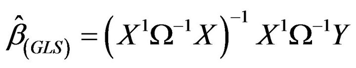
 , the resulting model is the Generalized Least Squares (GLS) Model. Aitken [15] has shown that the GLS estimator β of β given as
 is efficient among the class of linear unbiased estimators of β with variance-covariance matrix of β given as
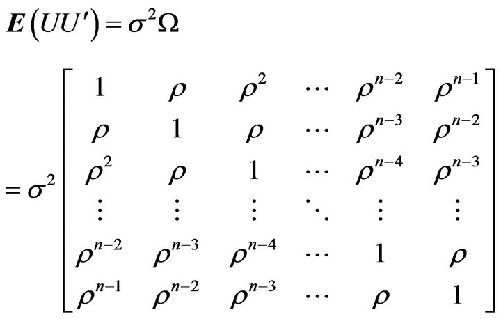
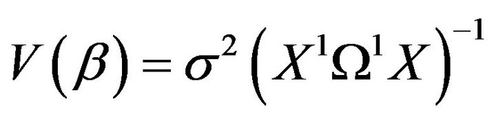 where Ω is assumed to be known. The GLS estimator described requires Ω, and in particular ρ to be known before the parameters can be estimated. Thus, in linear model with autocorrelated error terms having AR(1):
and
 (4)
(4)
where
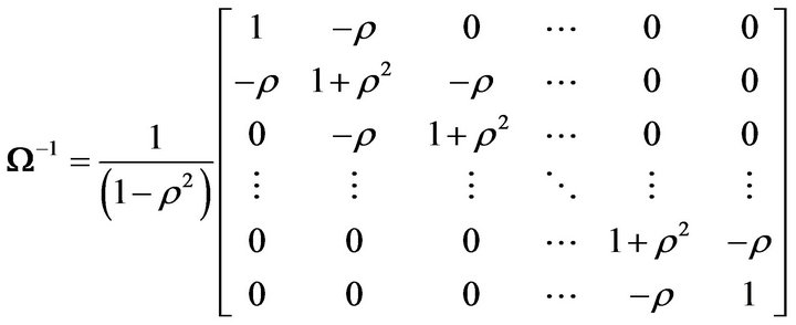
and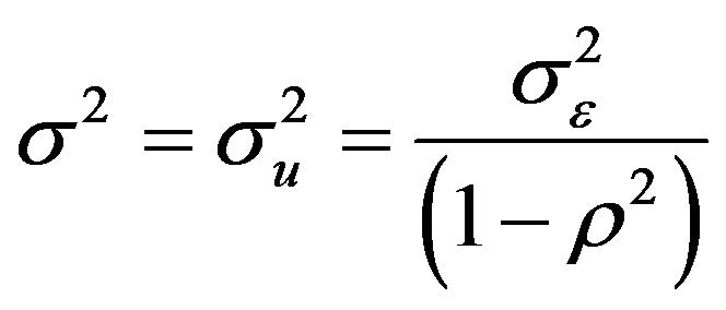 , and the inverse of Ω is
Now with a suitable  xn matrix transformation
  defined by
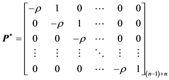 (5)
(5)
Multiplying then shows that  gives an n × n matrix which, apart from a proportional constant, is identical with
  except for the first elements in the leading diagonal, which is
  rather than unity. With another n × n transformation matrix P obtained from
by adding a new row with  in the first position and zero elsewhere, that is
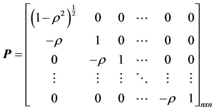 (6)
(6)
Multiplying shows that . The difference between
  and P lies only in the treatment of the first sample observation. However, when n is large, the difference is negligible, but in small sample, the difference can be major. If Ω or more precisely ρ is known, the GLS estimation could be achieved by applying the OLS via the transformation matrix
  and P above. However, this is not often the case; we resort to estimating Ω to have a Feasible Generalized Least Squares Estimator. This estimator becomes feasible when ρ is replaced by a consistent estimator
  [3]. There are several ways of consistently estimating ρ, however, some of them either use the
  or P transformation matrix.
Several authors have worked on this violation especially in terms of the parameters’ estimation of the linear regression model with autoregressive of orders one. The OLS estimator is inefficient even though unbiased. Its predicted values are also inefficient and the sampling variances of the autocorrelated error terms are known to be underestimated causing the t and the F tests to be invalid [3-5] and [16]. To compensate for the loss of efficiency, several feasible GLS estimators have been developed. These include the estimator provided by Cochrane and Orcutt [17], Paris and Winstern [18], Hildreth and Lu [19], Durbin [20], Theil [21], the Maximum Likelihood and the Maximum Likelihood Grid [22], and Thornton [23]. Among others, the Maximum Likelihood and Maximum Likelihood Grid impose stationary by constraining the serial correlation coefficient to be between –1 and 1 and keep the first observation for estimation while that of Cochrane and Orcutt and Hildreth and Lu drops the first observation. Chipman [24], Kramer [25], Kleiber [26], Iyaniwura and Nwabueze [27], Nwabueze [28-30], Ayinde and Ipinyomi [31] and many other authors have not only examined these estimators but have also noted that their performances and efficiency depend on the structure of the regressor used. Rao and Griliches [32] did one of the earliest Monte-Carlo investigations on the small sample properties of several two-stage regression methods in the context of autocorrelated error terms. Other recent works done on these estimators and the violations of the assumptions of classical linear regression model include that of Ayinde and Iyaniwura [33], Ayinde and Oyejola [34], Ayinde [35], Ayinde and Olaomi [36], Ayinde and Olaomi [37] and Ayinde [38].
In spite of these several works on these estimators, none has actually been done on prediction especially as it relates multicollinearity problem. Therefore, this paper does not only examine the predictive ability of some of these estimators but also does it under some violations of assumption of regression model making the model much closer to reality.
2. Materials and Methods
Consider the linear regression model of the form:
 (7)
(7)
where 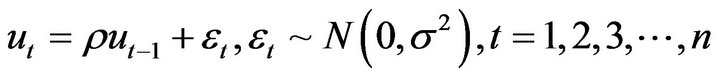 and
and  are stochastic and correlated.
For Monte-Carlo simulation study, the parameters of equation (1) were specified and fixed as β0 = 4, β1 = 2.5, β2 = 1.8 and β3 = 0.6. The levels of intercorrelation (multicollinearity) among the independent variables were sixteen (16) and specified as:
The levels of autocorrelation is twenty-one (21) and are specified as  Furthermore, the experiment was replicated in 1000 times
  under six (6) levels of sample sizes
 . The correlated stochastic normal regressors were generated by using the equations provided by Ayinde [39] and Ayinde and Adegboye [40] to generate normally distributed random variables with specified intercorrelation. With
 , the equations give:
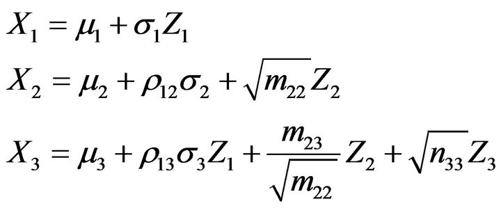 (8)
(8)
where 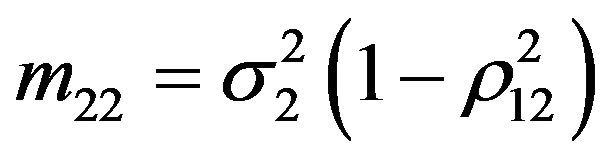 ,
, 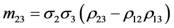 and
and 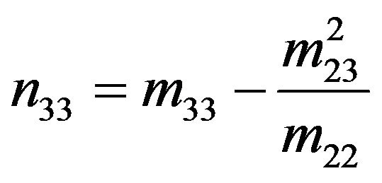 ; and
; and 
By these equations, the inter-correlation matrix has to be positive definite and hence, the correlations among the independent variables were taken as prescribed earlier
 . In the study, we assumed
The error terms were generated using one of the distributional properties of the autocorrelated error terms
 and the AR(1) equation as follows:
 (9)
(9)
 (10)
(10)
Since some of these estimators have now been incorporated into the Time Series Processor (TSP 5.0) [41] software, a computer program was written using the software to examine the goodness of fit statistics of the estimators by calculating their Adjusted Coefficient of Determination of the model . The estimators are Ordinary Least Square (OLS), Cochrane Orcutt (COR), Maximum Likelihood (ML) and the estimator based on Principal Component (PC) Analysis.The two possible PCs (PC1 and PC2) of the Principal Component Analysis were used. The Adjusted Coefficient of Determination of the model was averaged over the numbers of replications. i.e.
 (11)
(11)
An estimator is the best if its Adjusted Coefficient of Determination is the closest to unity.
3. Results and Discussion
The full summary of the simulated results of each estimator at different level of sample size, muticollinearity, and autocorrelation is contained in the work of Apata [42]. The graphical representations of the results when n = 10, 15, 20, 30, 50 and 100 are respectively presented in Figures 1, 2, 3, 4, 5 and 6.
From these figures, it is observed that the performances of COR at each level of multicollinearity and those of ML, especially when the sample size is large, over the levels of autocorrelation have a convex-like pattern, while those of OLS, PC1 and PC2 are generally concave-like. Also, as the level of multicollinearity increases the estimators, except PC estimators when multicolinearity is negative, rapidly perform better as their averaged adjusted coefficient of determination increases over the levels of autocorrelation. The PC estimators perform better as multicollinearity level increases in its
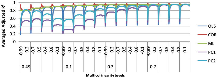
Figure 1. Predictive ability of the estimators at each level of multicollinearity and all levels of autocorrelation when n = 10.
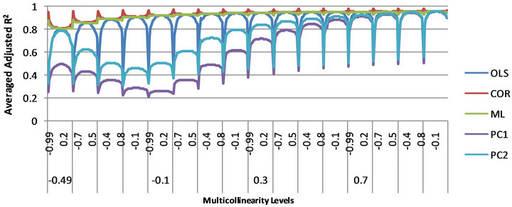
Figure 2. Predictive ability of the estimators at each level of multicollinearity and all levels of autocorrelation when n = 15.
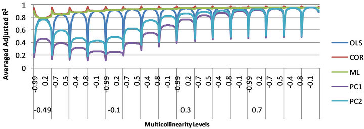
Figure 3. Predictive ability of the estimators at each level of multicollinearity and all levels of autocorrelation when n = 20.
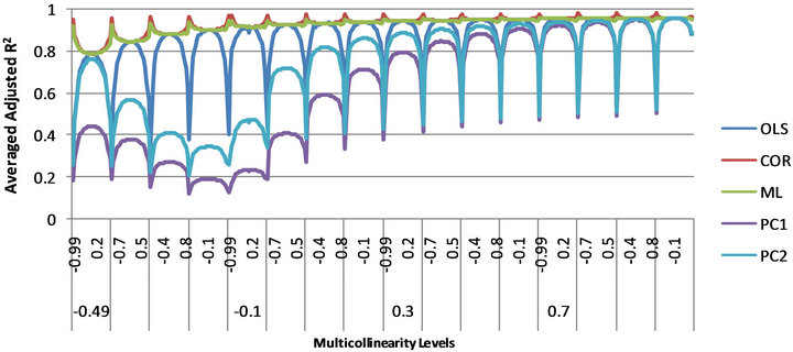
Figure 4. Predictive ability of the estimators at each level of multicollinearity and all levels of autocorrelation when n = 30.
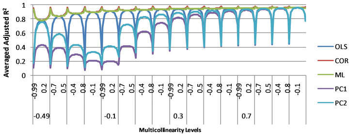
Figure 5. Predictive ability of the estimators at each level of multicollinearity and all levels of autocorrelation when n = 50.

Figure 6. Predictive ability of the estimators at each level of multicollinearity and all levels of autocorrelation when n = 100.
absolute value. The COR and ML estimators are generally good for prediction in the presence of multicollinearity and autocorrelated error term. However, at low levels of autocorrelation, the OLS estimator is either best or competes consistently with the best estimator, while the PC2 estimator is also either best or competes with the best when multicollinearity is high  .
.
Specifically, according to Figure 1 when n = 10, the average adjusted co-efficient of determination of the ML and COR estimators is often greater than 0.8. The OLS estimator consistently performs well and competes with the ML and COR estimators at low and occasionally at moderate levels of autocorrelation in all the levels of multicollinearity. Also, the PR1 and PR2 do perform well and compete with ML and COR except at high and very high level of autocorrelation when . The best estimator for prediction is summarized in Table 1.
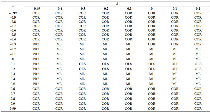
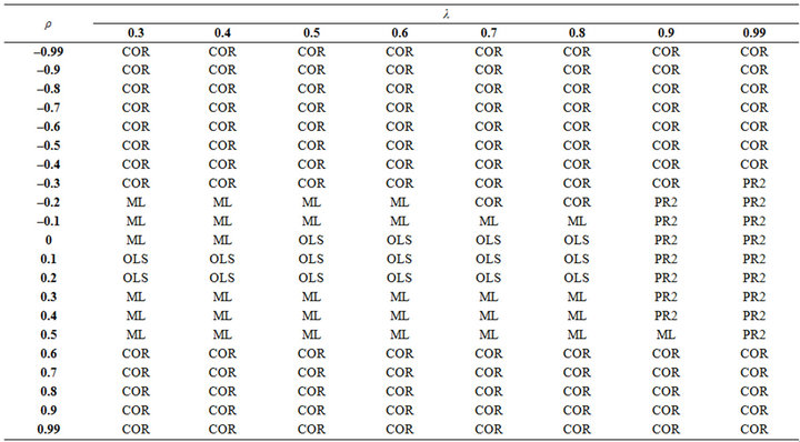
Table 1. The best estimator for prediction at different level of multicollinearity and autocorrelation when n = 10.
From Table 1, when n = 10, the COR estimator is best except when . At these instances, the PC2 estimator is often best when
  and
and  Moreover, when
  and
and , the OLS estimator is generally best. At other instances, the best estimator is frequently ML and very sparsely COR.
When n = 15, Figure 2 reveals that the pattern of the results is not different from when n = 10 except that PR estimators now compete very well with the ML and COR when . The best estimator for prediction is presented in Table 2.
According to Table 2, the COR estimator is generally
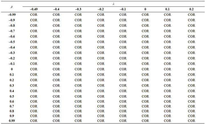
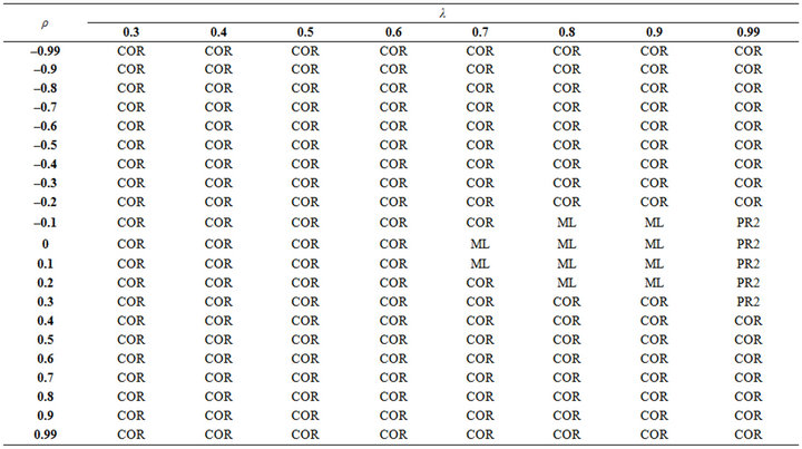
Table 2. The best estimator for prediction at different level of multicollinearity and autocorrelation when n = 15.
best except when . At these instances, the PC2 estimator is best when
  and at other instances, the best estimator is frequently ML or COR.
When n = 20, 30, 50 and 100, the results according to Figures 3, 4, 5 and 6 are not too different. However, from Table 3 when n = 20, the COR estimator is generally best except when . At these instances, the PC2 estimator is best when
  and
and . At other instances, the ML or COR is best.
When n = 30 from Table 4, COR estimator is gener-

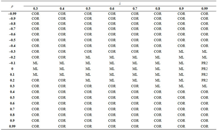
Table 3. The best estimator for prediction at different level of multicollinearity and autocorrelation when n = 20.
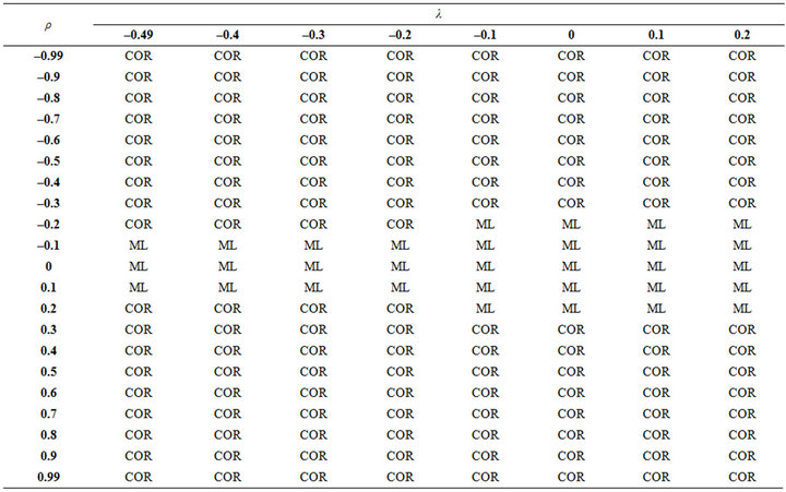
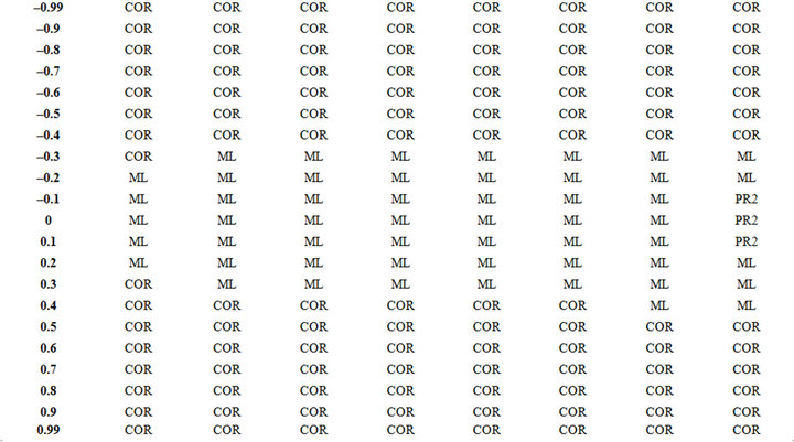
Table 4. The best estimator for prediction at different level of multicollinearity and autocorrelation when n = 30.
ally best except when . At these instances, the PC2 estimator is best when
 . At other instances, the best estimator is frequently ML and sparsely COR.
From Table 5 when n = 50, COR estimator is generally best except when . At these
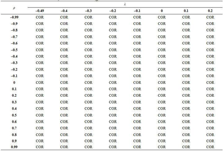
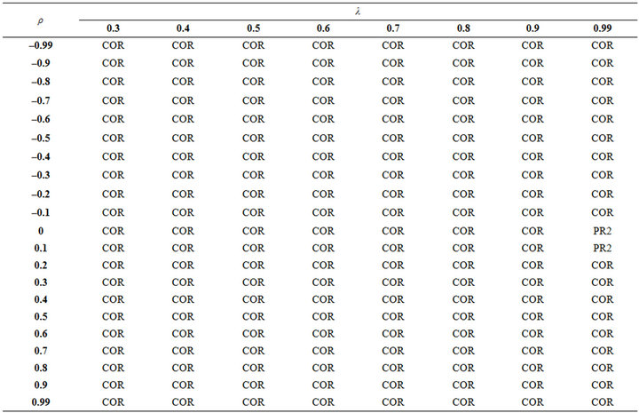
Table 5. The best estimator for prediction at different level of multicollinearity and autocorrelation when n = 50.
instances, the PC2 estimator is best. When n = 100 from Table 6, COR estimator is generally best.
4. Conclusion
The performances COR, ML, OLS and PCs estimators in prediction have been critically examined under the violation of the assumptions of fixed regressors, independent regressors and error terms. The paper has not only generally revealed how the performances of these estimators are affected by multicollinearity, autocorrelation and sample sizes but has also specifically identified the best estimator for prediction purpose. The COR and ML are

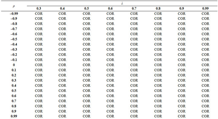
Table 6. The best estimator for prediction at different level of multicolli nearity and autocorrelation when n = 100.
generally best for prediction. At low levels of autocorrelation, the OLS estimator is either best or competes consistently with the best estimator while the PC2 estimator is either best or competes also with the best when multicollinearity level is high.
REFERENCES
- D. N. Gujarati, “Basic Econometric,” 4th Edition, Tata McGraw-Hill Publishing Company Limited, New Delhi and New York, 2005.
- J. Neter and W. Wasserman, “Applied Linear Model,” Richard D. Irwin Inc., 1974.
- T. B. Formby, R. C. Hill and S. R. Johnson, “Advance Econometric Methods,” Springer-Verlag, New York, Berlin, Heidelberg, London, Paris and Tokyo, 1984.
- G. S. Maddala, “Introduction to Econometrics,” 3rd Edition, John Willey and Sons Limited, Hoboken, 2002.
- S. Chartterjee, A. S. Hadi and B. Price, “Regression by Example,” 3rd Edition, John Wiley and Sons, Hoboken, 2000.
- A. E. Hoerl, “Application of Ridge Analysis to Regression Problems,” Chemical Engineering Progress, Vol. 58, No. 3, 1962, pp. 54-59.
- A. E. Hoerl and R. W. Kennard “Ridge Regression Biased Estimation for Non-Orthogonal Problems,” Technometrics, Vol. 8, No. 1, 1970, pp. 27-51.
- W. F. Massy, “Principal Component Regression in Exploratory Statistical Research,” Journal of the American Statistical Association, Vol. 60, No. 309, 1965, pp. 234- 246.
- D. W. Marquardt, “Generalized Inverse, Ridge Regression, Biased Linear Estimation and Non-Linear Estimation,” Technometrics, Vol. 12, No. 3, 1970, pp. 591-612.
- M. E. Bock, T. A. Yancey and G. G. Judge, “The Statistical Consequences of Preliminary Test Estimators in Regression,” Journal of the American Statistical Association, Vol. 68, No. 341, 1973, pp. 109-116.
- T. Naes and H. Marten, “Principal Component Regression in NIR Analysis: View Points, Background Details Selection of Components,” Journal of Chemometrics, Vol. 2, No. 2, 1988, pp. 155-167.
- I. S. Helland “On the Structure of Partial Least Squares Regression,” Communication Is Statistics, Simulations and Computations, Vol. 17, No. 2, 1988, pp. 581-607.
- I. S. Helland “Partial Least Squares Regression and Statistical Methods,” Scandinavian Journal of Statistics, Vol. 17, No. 2, 1990, pp. 97-114.
- A. Phatak and S. D. Jony, “The Geometry of Partial Least Squares,” Journal of Chemometrics, Vol. 11, No. 4, 1997, pp. 311-338.
- A. C. Aitken, “On Least Square and Linear Combinations of Observations,” Proceedings of Royal Statistical Society, Edinburgh, Vol. 55, 1935, pp. 42-48.
- J. Johnston, “Econometric Methods,” 3rd Edition, McGraw Hill, New York, 1984.
- D. Cochrane and G. H. Orcutt, “Application of Least Square to Relationship Containing Autocor-Related Error Terms,” Journal of American Statistical Association, Vol. 44, No. 245, 1949, pp. 32-61.
- S. J. Paris and C. B. Winstein “Trend Estimators and Serial Correlation,” Unpublished Cowles Commission, Discussion Paper, Chicago, 1954.
- C. Hildreth and J. Y. Lu, “Demand Relationships with Autocorrelated Disturbances,” Michigan State University, East Lansing, 1960.
- J. Durbin, “Estimation of Parameters in Time Series Regression Models,” Journal of Royal Statistical Society B, Vol. 22, No. 1, 1960, pp. 139-153.
- H. Theil, “Principle of Econometrics,” John Willey and Sons, New York, 1971.
- C. M. Beach and J. S. Mackinnon, “A Maximum Likelihood Procedure Regression with Autocorrelated Errors,” Econometrica, Vol. 46, No. 1, 1978, pp. 51-57.
- D. L. Thornton, “The Appropriate Autocorrelation Transformation When Autocorrelation Process Has a Finite Past,” Federal Reserve Bank St. Louis, 1982, pp. 82-102.
- J. S. Chipman, “Efficiency of Least Squares Estimation of Linear Trend When Residuals Are Autocorrelated,” Econometrica, Vol. 47, No. 1, 1979, pp. 115-127.
- W. Kramer, “Finite Sample Efficiency of OLS in Linear Regression Model with Autocorrelated Errors,” Journal of American Statistical Association, Vol. 75, No. 372, 1980, pp. 1005-1054.
- C. Kleiber, “Finite Sample Efficiency of OLS in Linear Regression Model with Long Memory Disturbances,” Economic Letters, Vol. 72, No. 2, 2001, pp.131-136.
- J. O. Iyaniwura and J. C. Nwabueze, “Estimators of Linear Model with Autocorrelated Error Terms and Trended Independent Variable,” Journal of Nigeria Statistical Association, Vol. 17, 2004, pp. 20-28.
- J. C. Nwabueze, “Performances of Estimators of Linear Model with Auto-Correlated Error Terms When Independent Variable Is Normal,” Journal of Nigerian Association of Mathematical Physics, 2005, Vol. 9, pp. 379-384.
- J. C. Nwabueze, “Performances of Estimators of Linear Model with Auto-Correlated Error Terms with Exponential Independent Variable,” Journal of Nigerian Association of Mathematical Physics, Vol. 9, 2005, pp. 385- 388.
- J. C. Nwabueze, “Performances of Estimators of Linear Model with Auto-Correlated Error Terms When the Independent Variable Is Autoregressive,” Global Journal of Pure and Applied Sciences, Vol. 11, 2005, pp. 131-135.
- K. Ayinde and R. A. Ipinyomi, “A Comparative Study of the OLS and Some GLS Estimators When Normally Distributed Regressors Are Stochastic,” Trend in Applied Sciences Research, Vol. 2, No. 4, 2007, pp. 354-359. doi:10.3923/tasr.2007.354.359
- P. Rao and Z. Griliches, “Small Sample Properties of Several Two-Stage Regression Methods in the Context of Autocorrelation Error,” Journal of American Statistical Association, Vol. 64, 1969, pp. 251-272.
- K. Ayinde and J. O. Iyaniwura, “A Comparative Study of the Performances of Some Estimators of Linear Model with Fixed and Stochastic Regressors,” Global Journal of Pure and Applied Sciences, Vo.14, No. 3, 2008, pp. 363- 369. doi:10.4314/gjpas.v14i3.16821
- K. Ayinde and B. A. Oyejola, “A Comparative Study of Performances of OLS and Some GLS Estimators When Stochastic Regressors Are Correlated with Error Terms,” Research Journal of Applied Sciences, Vol. 2, No. 3, 2007, pp. 215-220.
- K. Ayinde, “A Comparative Study of the Perfomances of the OLS and Some GLS Estimators When Stochastic Regressors Are both Collinear and Correlated with Error Terms,” Journal of Mathematics and Statistics, Vol. 3, No. 4, 2007, pp. 196-200.
- K. Ayinde and J. O. Olaomi, “Performances of Some Estimators of Linear Model with Autocorrelated Error Terms when Regressors are Normally Distributed,” International Journal of Natural and Applied Sciences, Vol. 3, No. 1, 2007, pp. 22-28.
- K. Ayinde and J. O. Olaomi, “A Study of Robustness of Some Estimators of Linear Model with Autocorrelated Error Terms When Stochastic Regressors Are Normally Distributed,” Journal of Modern Applied Statistical Methods, Vol. 7 No. 1, 2008, pp. 246-252.
- K. Ayinde, “Performances of Some Estimators of Linear Model When Stochastic Regressors are Correlated with Autocorrelated Error Terms,” European Journal of Scientific Research, Vol. 20 No. 3, 2008, pp. 558-571.
- K. Ayinde, “Equations to Generate Normal Variates with Desired Intercorrelation Matrix,” International Journal of Statistics and System, Vol. 2, No. 2, 2007, pp. 99-111.
- K. Ayinde and O. S. Adegboye, “Equations for Generating Normally Distributed Random Variables with Specified Intercorrelation,” Journal of Mathematical Sciences, Vol. 21, No. 2, 2010, pp. 83-203.
- TSP, “Users Guide and Reference Manual,” Time Series Processor, New York, 2005.
- E. O. Apata, “Estimators of Linear Regression Model with Autocorrelated Error term and Correlated Stochastic Normal Regressors,” Unpublished Master of Science Thesis, University of Ibadan, Ibadan, 2011.