Open Journal of Statistics
Vol.1 No.2(2011), Article ID:6551,11 pages DOI:10.4236/ojs.2011.12015
Fibonacci Congruences and Applications
Laboratory LJK, Université Joseph Fourier, Grenoble, France
E-mail: rene.blacher@aliceadsl.fr
Received May 24, 2011; revised June 14, 2011; accepted June 20, 2011
Keywords: Fibonacci Sequence, Linear Congruence, Random Numbers, Dependence, Correct Models
Abstract
When we study a congruence T(x) ≡ ax modulo m as pseudo random number generator, there are several means of ensuring the independence of two successive numbers. In this report, we show that the dependence depends on the continued fraction expansion of m/a. We deduce that the congruences such that m and a are two successive elements of Fibonacci sequences are those having the weakest dependence. We will use this result to obtain truly random number sequences xn. For that purpose, we will use non-deterministic sequences yn. They are transformed using Fibonacci congruences and we will get by this way sequences xn. These sequences xn admit the IID model for correct model.
1. Introduction
In this paper, we present a new method using Fibonacci sequences to obtain real IID sequences  of random numbers1. To have random number two methods exists : 1) use of pseudo-random generators (for example the linear congruence), 2) use of random noise (for example Rap music).
But, up to now no completely reliable solution had been proposed ([1]-[3]). To set straight this situation, Marsaglia has created a Cd-Rom of random numbers by using sequences of numbers provided by Rap music. But, he has not proved that the sequence obtained is really random.
However, by using Fibonacci congruence, there exists simple means of obtaining random sequences whose the quality is sure (cf [4]): one uses the same method as Marsaglia, but one transforms the obtained sequence by Fibonacci congruences. Then, one obtains sequence of real xnsuch that the IID model is a correct model of xn.
1.1. Fibonacci Congruence
Linear congruences  mod (m) are often used as pseudo-random generators. In this case, we try to choose a and m so that successive pseudorandom numbers behave as independent. Of course, we can only ensure that it is the case of p successive numbers p where
 . To choice a and m, one can use the spectral test or the results of Dieter (cf [5]) which allow to choose the best “a”.
Unfortunately, the conditions which ensure the independence of three successive numbers are not those which ensure the best independence of two successive numbers,for example.
Indeed, in this paper, we will study the conditions which ensure the independence of only two successive numbers and we will see with astonishment that this is the Fibonacci congruence which provides the best empirical independence.
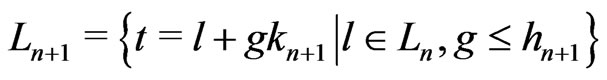
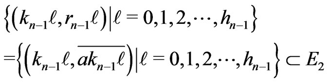
We shall study the set
 when
when  modulo m and
  if
if . We will understand that this dependence depends on the continued fraction
 i.e. it depends on sequences
  and
and  defined in the following way.
Notations 1.1 Let ,
, . One denotes by
  the sequence defined by
  the Euclidean division of
  by
by  when
when . Moreover, one denotes by d the smallest integer such as
 . One sets
 .
.
One sets ,
,  and
and  if
if .
.
Then, dependence depends on the ’s: more they are small, more the dependence is weak.
Theorem 1 Let . Let
. Let  and let
 , be the rectangle
  modulo m. Then If n is even,
 . Moreover the points
  are lined up modulo m.
If n is odd,
 .
.
Moreover, the points  are lined up modulo m.
Of course, in general, it is only on the border that , the rectangle modulo m, satisfies
 . If not,
  is a normal rectangle.
For example if , this theorem means that the rectangle
  does not contain points of
  if n is even:
 . If
. If  is large, that will mean that an important rectangle of
  is empty of points of
 : that will mark a breakdown of independence.
As , the congruence which defines the best independence of
  will satisfy
  and
and . In this case we call it congruence of Fibonacci. Indeed, there exists
  such that
  and
and  where
where  is the sequence of Fibonnacci:
 ,
, . As a matter of fact the sequence
  is the sequence of Fibonacci except for the last terms (i.e. except for
 ). It is also the case for sequence
 .
.
Remark 1.1 In fact, when we use sequence , we use Euclidean Algorithm. Now, Dieter has also used this algorithm to compute the dependence of
  when
when . But he has not understood the part of the
 ’s in this dependence.
1.2. Application: Building of Random Sequence
Unfortunately, congruences of Fibonacci cannot be used in order to directly generate good pseudo random sequences because  where
where  is the identity (cf page 141 of [6]). Indeed in this case, the pseudo random sequence
  checks
 . However, one can use congruence of Fibonacci in order to build IID sequences by transforming some random noise
 .
.
Definition 1.2 Let . Let T be the congruence of Fibonacci modulo m. We define the function of Fibonacci
  by
by  where
where
1)
2)  when
when  is the binary writing of z.
We choose , n = 1, 2,
 ,N. Then,
  admits for correct model a sequence of random variables
  defined on a probability space
 . Then, we will impose to
  that the conditional probabilities of
  admit densities with Lipschitz coefficient bounded by
  not too large.
In fact, since  has discrete value, we can always assume that
  has a continuous density.
Notations 1.3 We denote by  be the uniform measure defined on
  by
by  for all
 .
.
For all permutation  of
of , for all
 , we denote by
  the conditional density with respect to
  of
of  given
given .
.
Since  is discrete, we can also assume that
  has a finite Lipschitz coefficient.
Notations 1.4 We denote by  a constant such that, for all permutation
  of
of , for all
 ,
, . In order to simplify the proofs we suppose
 .
.
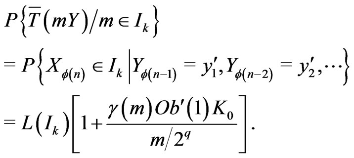
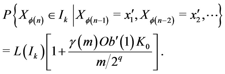
Now, we shall prove easily that the conditional probabilities of  check
check
Then we shall choose m and q such that  is small enough. We shall deduce that, for all Borel set
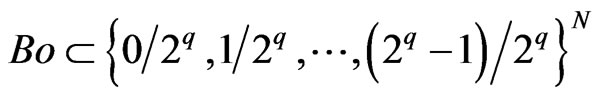 ,
,
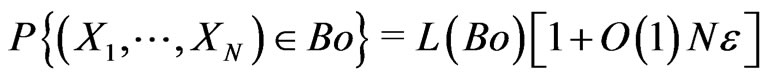 where L is the measure corresponding to the Borel measure in the case of discrete space :
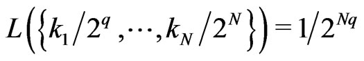 .
.
Then  cannot be differentiated from an IID sequence. Indeed, it is wellknown that, for a sample
 , there is many models correct : in particular, if
  is extracted of an IID sequence, models such that
  are correct if
  is small enough with respect to N. Reciprocally, if the sequence of random variables
  checks
 , the model IID is also a correct model for the sequence
 .
.
Thus one will be able to admit that the IID model is a correct model for the sequences . As a matter of fact, one will be even able to admit that there exists another correct model
  of
of  such that
  is exactly the IID sequence.
Now there exists noises  such that
  is not too large. For example these sequences can be built by using texts. In this case we can prove the result : in order that
  is IID, it suffices that
  admits a correct model such that
  is not too large. However, it is a condition which can be imposed easily by transforming some noises. The advantage compared with the CD-Rom of Marsaglia is that this result is proved. Of course, we tested such sequences.
So finally we can indeed build sequences  admitting for correct model the IID model by using Fibonacci congruences. This means that, a priori, these sequences
  behave as random sequences. It is always possible that they do not satisfy certain tests. But it will be a very weak probability as we know it is the case for samples of sequences of IID random variables.
We point out that a first version of these results are in [4]. Moreover, all these results and the proofs are detailed in [7].
Note that to use the congruence of Fibonacci method is completely different from the method using Fibonacci sequence with  modulo m, which is moreover a bad generator : cf page 27 of [1].
2. Dependence Induced by Linear Congruences
In this section, we study the set  when T is a congruence
  modulo m.
2.1. Notations
We recall that we define sequences  and
and  by the following way: we set
 ,
,  and
and , the Euclidean division of
  by
by  when
when . One denotes by d the smallest integer such as
 . One sets
 . Moreover,
  ,
,  and
and  if
if .
.
Then 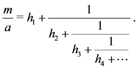
Therefore,  for all n = 1, 2,
 ,d and
 . The full sequence
  is thus the sequence
 ,
,  ,
, ,
, ,
, . Then, if T is a Fibonacci conguence,
  is the Fibonacci sequence
 , except for the last terms.
Remark that if  for n = 1,2,
 ,d – 1,
  is also the Fibonacci sequence for n = 1,2,
 ,d. Indeed by definition,
  ,
,  and
and  if
if .
.
2.2. Theorems
Now, in order to prove the theorem 1, it is enough to prove the following theorem.
Theorem 2 Let . Then
If n is even, . Moreover the points
  are lined up.
If n is odd,
 .
.
Moreover, the points 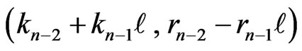 are lined up.
Then, if there exists  large, there is a breakdown of independence. For example if n = 2, it is a wellknown result. Indeed,
  ,
,  ,
,  and
and  where
where  means the integer part of x. Thus, the rectangle
  will not contain any point of
 . However, this rectangle has its surface equal to
 . Thus if “a” is not sufficiently large, i.e if
  is too large, there is breakdown of independence.
We confirm by graphs the previous conclusion. We suppose m = 21. If a = 13, we have a Fibonacci congruence: cf Figure 1. If one chooses a = 10, : cf Figure 2 . If one chooses a = 5,
 : cf Figure 3.
Then, in order to avoid any dependence, it is necessary that  is small.
2.3. Distribution of T([c,c'[) When T Is a Fibonacci Congruence
We assume that T is a Fibonacci congruence. Let  where
where .
.
We are interested by  or
or  because
 . Since
  behaves as independent of I, normally, we should find that
  and, therefore
 , is well distributed in
 . As a matter of fact it is indeed the case.
Indeed, let , n = 1, 2,
 , c' – c, be a permutation of
  such that
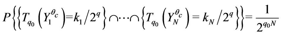
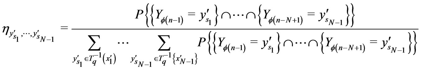
 . Thenfor all numerical simulations which we executed, one has always obtained
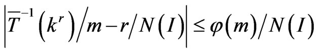
where . In fact, it seems that
  is of the order of Log(Log(m)). Moreover,
  seems maximum when I is large enough :
 .
.
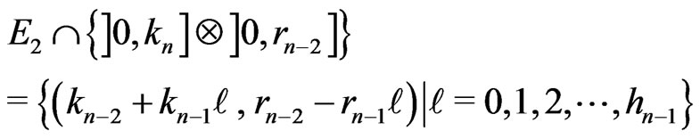
For example, in Figures 4, 5 and 6, we have the graphs , r = 0, 1,
 ,N(I) – 1 for
Figure 1. Fibonacci congruence.
Figure 2. sup(hi) = 20.
Figure 3. sup(hi) = 5.
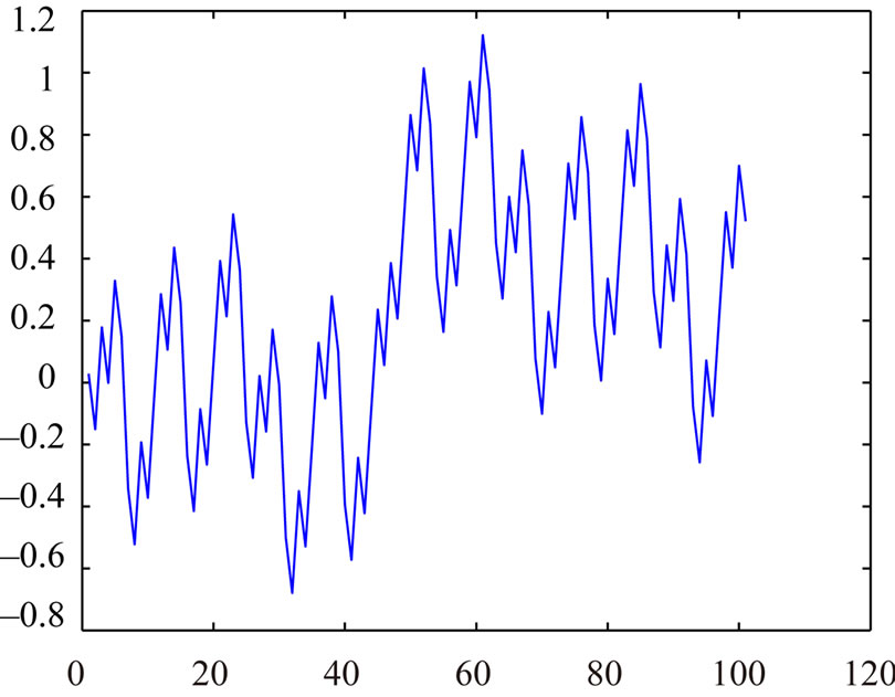
Figure 4. a = 1346269, m = 2178309.
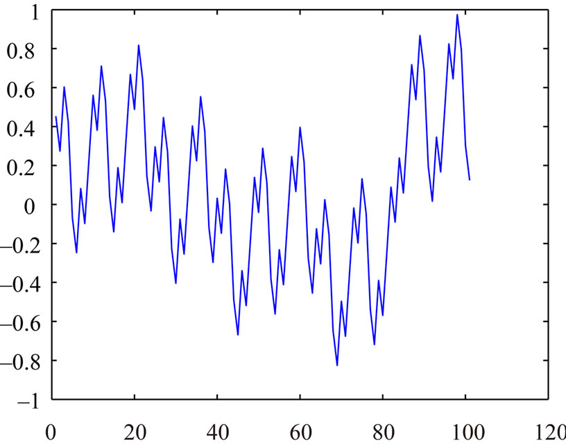
Figure 5. a = 121393, m = 196418.
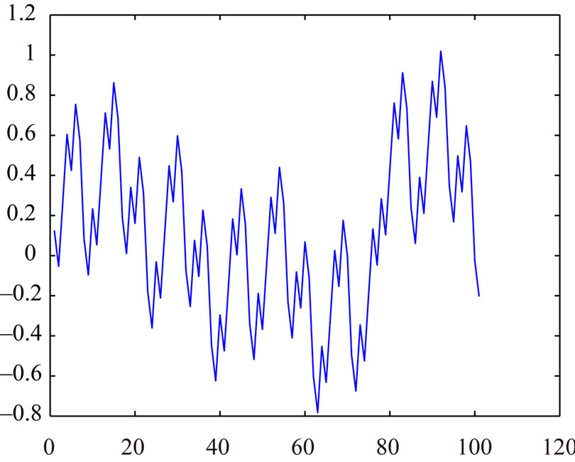
Figure 6. a = 10946, m = 17711.
various Fibonacci congruences when c' – c = 100.
3. Proof of Theorem 2
In this section, the congruences are conguences modulo m. Now the first lemma is obvious.
Lemma 3.1 For n = 3,4, ,d + 1,
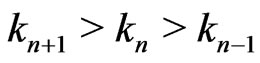 . Moreover
  is the Euclidean division of
  by
by .
.
Now, we prove the following results.
Lemma 3.2 Let n = 0, 1, 2 , , d. If n is even,
 . If n is odd,
 .
.
Proof. We prove this lemma by recurrence. For n = 0,
 . For n = 1,
 .
.
We suppose that it is true for n.
One supposes n even. Then, .
.
One supposes n odd. Then, .
.
Therefore, .
.
Lemma 3.3 Let n = 2,3, ,d + 1. Let
 . If
. If  is even,
 .
.
If  is odd,
 .
.
Moreover, if  is even,
 . If
. If 
is odd, .
.
Proof. The second assertion is lemma 3.2. Now, we prove the first assertion by recurrence.
One supposes n = 2. Then, . Moreover,
 . If
. If ,
, .
.
If ,
, . In this case, we study
  where
where . Then,
 . Then,
 .
.
Moreover,
 .
.
Therefore, because ,
, .
.
Therefore, .
.
One supposes that the first assertion is true for n where .
.
Let . Let
. Let  be the Euclidean division of t' by
 :
: .
.
Then, . If not,
 .
.
One supposes n even.
In this case,  for
for
 .
.
Moreover, .
.
First, one supposes . Then,
 .
.
Moreover, because ,
,
 .
.
Therefore, because ,
, .
.
Therefore, .
.
Now, one supposes  and
and .
.
By recurrence,
 .
.
Therefore, because ,
, .
.
Therefore, .
.
One supposes ,
,  and
and .
.
If ,
, . Indeed, if not,
 . For example, if
 ,
, . Then, because our recurence,
 : it is impossible.
Now, if ,
, .
.
Moreover, if ,
, . Then, by recurence
 .
.
Then, if ,
, . Then,
 .
.
Moreover,
 .
.
Therefore, because ,
, .
.
Therefore, .
.
One supposes  and
and . Then,
 . It is opposite to the assumption.
Then, in all the cases, for ,
,
 . Therefore, the lemma is true for n + 1 if n is even. Then, it is also true for n + 1 = 3.
One supposes n odd with . One proves the recurrence by the same way as if n is even (cf [7]). Then the lemma is true for n+1.
Lemma 3.4 The following inequalities holds: .
.
Proof. If , by lemma 3.3,
 or
or , i.e.
  or
or  where
where . Then,
  or
or .
.
Then, if , there exists
such that , i.e.
 . It is impossible.
Lemma 3.5 Let  such that
 . Then, t=t'.
Proof. Suppose . Then,
  and
and . Then, by lemma 3.3,
 or
or 
where . Then,
 . It is a contradiction.
Lemma 3.6 Let n = 1, 2, ,d. Let
 . Then,
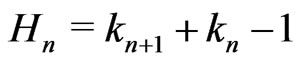
The proof is basic.
Lemma 3.7 Let n = 1, 2, 3, ..., d – 1 . Let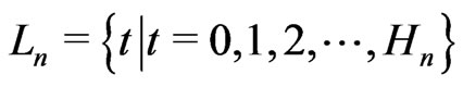 . Then, for all
 ,
,
 .
.
Proof. Let ,
, . Let
. Let . Therefore, if
 ,
, . Therefore,
 .
.
Reciprocally, let  and let
 ,
,  be the Euclidean division of t by
 .
.
We know that . Therefore,
 . Therefore,
 .
.
Therefore, if ,
,
 .
.
Moreover, if ,
,
 .
.
Therefore, .
.
Then, suppose . Then,
 .
.
Because  and
and ,
, . Therefore,
 .
.
Therefore,  where
where 
Therefore,  where
where .
.
Therefore,  .
.
Therefore, .
.
Therefore, .
.
Lemma 3.8 Let .
.
Let . We set
 where
where  and
and  for all
 .
.
Then, for all ,
,  or
or .
.
Proof We prove this lemma by recurrence.
Suppose n = 1. Then,  ,
, . Therefore,
 .
.
Therefore, the lemma is true for n = 1.
Suppose that the lemma is true for n.
Then, 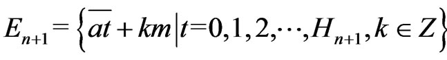 , where
 .
.
Because ,
, . By lemma 3.7, If
 ,
,  where
where . By lemma 3.2,
 .
.
Therefore,
Suppose that n is even.
Then,  because
 .
.
Use the recurrence. Suppose . Then,
 .
.
Therefore,
 .
.
Therefore,  or
or  if
if .
.
Suppose . Then, s is fixed .
Let . Therefore,
 .
.
Let .
.
Then, .
.
Therefore,  where
where . Moreover,
 .
.
Therefore, if  and
and 
 or
or .
.
Suppose that n is odd. One proves this result by the same way as when n is even (cf [7]).
Proof 3.9 Now one proves theorem 2.
Suppose that n is even.
Then,  ,
,  , ......
 .
.
Now,  for
for .
.
 Therefore,
Moreover, . On the other hand, by lemma 3.8 , all the points of
 ,
,  , have ordinates distant of
  or
or .
.
Therefore, if there is other points of  that the points
 , there exists
 and
and  such that
 .
.
Because , by lemma 3.5, there exists an only
 , such that
 :
: . Because
 , there exists an only
 , such that
 .
.
Now, . Then,
 .
.
Then, .
.
Because  with
with ,
, . Moreover,
 . Then,
 . Then,
 .
.
Then, by lemma 3.4,
 . Then,
 .
.
Then, by lemma 3.4,
 .
.
Then, .
.
Now . Moreover,
 .
.
Then, because , by lemma 3.5,
 .
.
Then, . It is a contradiction.
Therefore, there is not other points of  that
that
 .
.
Therefore, there is not other points of  that the points
 .
.
Therefore,

According to what precedes,
is located on the straight line  if n is even.
Suppose that n is odd. One proves this result by the same way as when n is even (cf [7]).
4. Models Equivalent with a Margin of 
4.1. Correct Models
In general terms, one can always suppose that  is the realization of a sequence of random variables
  defined on a probability space
 :
:  where
where  and where
  is a correct model of
 . As a matter of fact, there exist an infinity of correct models of
 . It is thus necessary to be placed in the set of all the possible random variables.
Notations 4.1 One considers the sequences of random variables , n = 1,
 ,N, defined on the probabilities spaces
 ,
, :
:
 . One assumes that
  for all
 .
.
For example, one can assume that  and
and .
.
It thus raises the question to define what is a correct model. Indeed, if a model  is not correct, it is however possible that
 . Now, in the case where the model
  is IID, to define a correct model is a generalization of the problem of the definition of an IID sequence. Then, it is a very complex problem (cf [1]).
However, generally, one feels well that correct models exist. In fact, it is a traditional assumption in science. In weather for example, the researchers seek a correct model, which implies its existence (if not, why to try to make forecasts?).
One could thus admit that like a conjecture or a postulate without defining exactly what is a correct model. Cependant, a more detailed study is in [7].
4.2. Models Equivalent
4.2.1. The Problem
Let  and
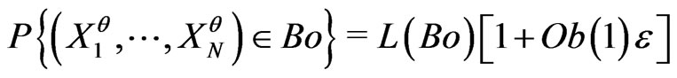
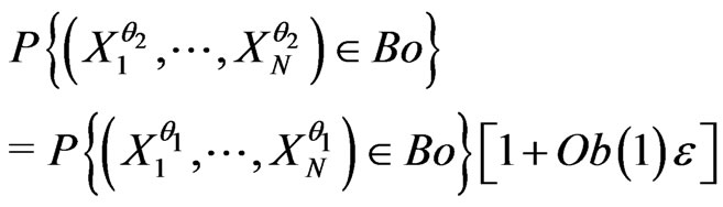
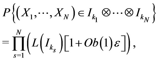
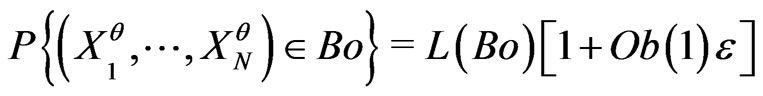
and  be two sequences of random variables such that, for all Borel set Bo,

where Ob(.) means the classical O(.) with the additional condition . One supposes that
  is a correct model of the sequence
 , n = 1, 2,
 ,N. One wants to prove that
  is also a correct model of
  if
if  is small enough.
4.2.2. Example
Let us suppose that we have a really IID sequence of random variables  with uniform distribution on [0,1/2] and [1/2,1] and with a probability such as
  where
where . Then, this sequence has not the uniform distribution on [0,1]. However, if we have a sample with size 10, we will absoluetely not understand that
  has not the uniform distribution on [0,1]. It is wellknown that one need samples with size larger than N = 1000 minimum in order to test this difference.
For example, one cannot test significantly : “
: “ has the uniform distribution” against
 :
:
“ ” if
” if .
.
Indeed, if  and b = 2, the probability of obtaining
 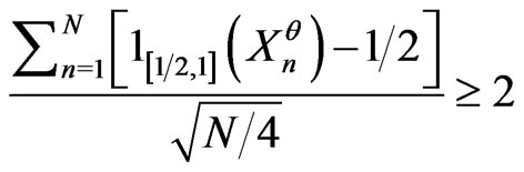 is about 0.0466 under
  and about 0.0455 under
 : i.e. the probability of rejecting the assumption IID,
  , under
  is not much bigger than that of rejecting
  if
if  is really IID (cf also section 4.3 of [8]).
Then it is no possible to differentiate the IID model and models such that
 .
.
4.2.3. Border of Correct Models
Now there is a problem : for example, use a realization  of the IID model, and let
  be a model checking
 where
where
 is small enough but not very small. Let
  be a model such that
 .
.
Then,  can be not a correct model: it is enough that
  is in extreme cases of the possible values of the
 ’s such that
 ,
,
 , imply that
  is a correct model.
Then, there are models more correct than others. These are models  such that, if
 ,
,  is also a correct model where
  is small enough, but not too small. For example,
  , 1/100 or at worst
  if need be (cf section 5-7 of [7]).
It seems clear that such models exist. For example it is assumed that this is the case when  is sample of an IID sequence
  and that it is a good realization of
 .
.
On the other hand, we know that it should exist estimates of models (these estimates are easier to calculate in some cases as texts). Then, we can choose as model , the model provided by these estimates : close models will also correct models.
All these points are detailed in [7].
4.3. Exact IID Model
Then, generally, if  is a correct model such that
  cannot be differentiated with the IID model, one will be able to choose another correct model
  close to
  and such that
  is exactly the IID model. Indeed one proves easily the following proposition (cf proposition 5-1 of [8]).
Proposition 4.1 One assumes that m is large enough. Let  be a correct model of the sequence
 . One assumes that there exists
  such that if
  is a model satisfying, for all Borel set Bo,
  , then
  is a correct model of
 .
.
One assumes also that, for all ,
,
where . One assumes that
  is increasing, that
  and that there exists
  such that
  is small enough.
Then, there exists  and a correct model
  of the sequence
  such that, for all
 ,
,
5. Approximation Theorem
5.1. Theorem
In this section, we assume that T is a Fibonacci congruence and we use Fibonacci function  in order to build IID sequences.
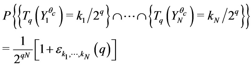
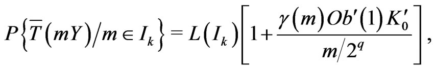
Theorem 3 We keep the notations 1.3 and 1.4 and notations of section 2.3. Let . We assume
  and
and . Then, for all Borel set Bo,
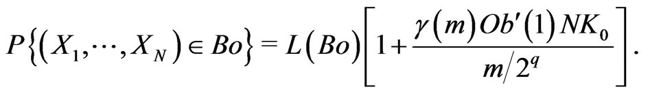
where  is increased by a number close to 1.
If  is not too large, there is no difficulty to choose m and q in such a way that
 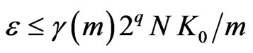 is small enough. Therefore,
 .
.
5.2. Proof
Because, by Section 2.3, the points of  are well distributed in
 , it is easy to prove that the sum of points of
  will be close
 (e.g. cf Figure 7). Then, we have the following lemma (cf also proposition 6-1 of [7]).
Lemma 5.1 Let  be the probability density function of
 , with respect to
 :
:
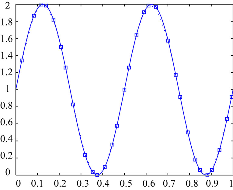
Figure 7. Points of  when
when .
.
 . Let
. Let  such that
 .
.
Let  such that
  and
and  when
when . One supposes
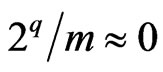 , and
, and 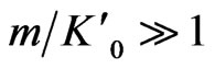 .
.
Then, the following equality holds:
where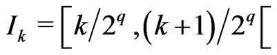 ,
, .
.
Then, one can prove theorem 3. Indeed, by applying lemma 5.1 when  has for distribution the distribution of the conditional probability of
  given
given , we have
Now, one proves easily that
where
Then, 
We deduce that
Then, one proves by basic methods (cf proposition 6.2 of [7]) that, for all ,
,
where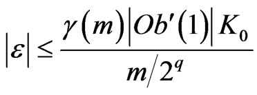 . Because
 , we deduce that
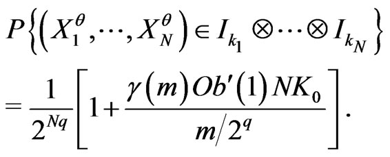
Now, we deduce that, for all Borel set
6. Choice of Random Noises
6.1. Use of Texts
Now, we suppose that we use sequences  and
and , n = 1,2,
 ,N, obtained from independent texts. In order to reduce
  we add modulo m a text and a text written backward:
 where
where  is pseudo-random sequences which have good empirical independence assumptions for p successive pseudo random numbers when
 . In an obvious way, the texts are realizations of sequences of random variables : for example, one can take as model, the set of the possible texts provided with the uniform probability As a matter of fact, we add
  to have sequences
  which have a good randomness (cf [9], or chapter 3 of [6]).
In particular, a priori, “ is not too different from 1/m” is a reasonable assumption. Moreover,
  has a empirical distribution close to independence and texts behaves as Q-dependent sequences (cf [6]). Then, for all permutation
 , a three-dimensional model
  with a continuous density and a Lipschitz coefficient not too big will be a good model. By the same way,
 is not too different of
  which is not too different from 1/m (cf [7]). In this case, one can prove that generally
  is small cf [7].
On the other hand, to increase  a good way is to use the Central Limit theorem. In fact one can combine the two methods : cf [7].
6.2. Example
Now it may be necessary to do some transformations to get the  in the case where the letters and symbols are provided by sequences a(j),
  ,
,  ,
, .
.
One sets . We choose two consecutive elements a and m of the Fibonacci sequence : m can be chosen with respect to
 . Then, we choose
  such that
 .
.
1) We set  mod
mod 
2) We set  for
for
 .
.
3) We set  for
for .
.
By using this technique, we have created real IIID sequences . We have used a sequence c(j) with
 . This sequence was obtained from dictionary, encyclopedia, and Bible. We choose
 ,
,  ,
, . Then
 . Then, we have estimated
 . In order to avoid any error we have choose
  in the building of
 .
.
We have tested the sequence . We have used the classical Diehard tests (cf [1] [2]) and the higher order correlation coefficients (cf [10]). Results are in accordance with what we waited: the hypothesis “randomness” is accepted by all these tests (cf [7]).
One can can download this sequence in [11]
7. Conclusion: Building of Random Sequence
By theorem 3 one can find models correct  such that
 where
where 
is small if  is not too large. Now it is possible to build such sequences concretely, for example by using texts studied in section 6. In this case, coefficient
  depend on the choice of m, i.e. of
 . But,
  increases very little when
  increases. Even, in some cases, it seems that it decreases. Then, at most
  decreases much more quickly than
  increases.
So by taking m large enough and by choosing well q, we found  small enough in a way that there exists correct models which checks the conditions of proposition 4.1. Then, there exists m sufficiently large and q sufficiently small and a correct model
  such that
  is the IID model.
Then, this result show that one can build sequences  such that the model IID is a correct model of
 .
.
That means that  behaves like any IID sample: a priori,
  can check not the properties which one expects from a IID sample like certain tests, but that occurs only with a probability equal to that of any IID sample.
By this method, we therefore have a mean to value the technique used by Marsaglia to create its CD-ROM. We arrive in fact to prove mathematically that the sequence obtained can be regarded a priori as random, what Marsaglia did not.
Remark 7.1 One might wonder if the sequence built adding text and pseudo-random sequences is not an lID sequence. It is a similar hypothesis which Marsaglia does when he built its CD-Rom. This also corresponds to results of [9]. But in fact, nothing is proved.
It is maybe possible to prove it but that seems complicated. Finally, it is much easier to apply the functions : in this case, it requires only that
  is not too big. It’s an hypothesis much simpler to be verified and it does not require many efforts in some cases. That is why we choose to build IID sequences using this technique.
8. References
[1] D. E. Knuth, “The Art of Computer Programming,” 3rd Edition, Addison-Wesley, Boston, 1998.
[2] J. Gentle, “Random Number Generation and Monte Carlo Method,” Springer 13, 1984, pp. 61-81.
[3] A. Menezes, P. Van Oorschot, S. Vanstone, “Handbook of Applied Cryptography,” CRC Press, London, 1996. doi:10.1201/9781439821916
[4] R. Blacher, “Solution Complete Au Probleme des Nombres Aleatoires,” 2004. http://www.agro-montpellier.fr/sfds/CD/textes/blacher1.pdf
[5] U. Dieter, “Statistical Interdependence of Pseudo Random numbers Generated by the Linear Congruential Method,” In: S. K. Zaremba, Ed., Applications of Number Theory to Numerical Analysis, Academic Press, New York, 1972, pp. 287-317.
[6] R. Blacher, “A Perfect Random Number Generator,” Rapport de Recherche LJK Universite de Grenoble, 2009. http://hal.archives-ouvertes.fr/hal-00426555/fr/
[7] R. Blacher, “Fibonacci Congruences and Applications,” Rapport de Recherche LJK Universite de Grenoble, 2011. http://hal.archives-ouvertes.fr/hal-00587108/fr/.
[8] R. Blacher, “Correct models,” Rapport de Recherche LJK Universite de Grenoble, 2010. http://hal.archives-ouvertes.fr/hal-00521529/fr/
[9] L. Y. Deng and E. O. George, “Some Characterizations of the Uniform Distribution with Applications to Random Number Generation,” Annals of the Institute of Statistical Mathematics, Vol. 44, No. 2, 1992, pp. 379-385. doi:10.1007/BF00058647
[10] R. Blacher, “Higher Order Correlation Coefficients,” Statistics, Vol. 25, No. 1, 1993, pp. 1-15. doi:10.1080/02331889308802427
[11] R. Blacher, File of random Number, 2009. http://www-ljk.imag.fr/membres/Rene.Blacher/GEAL/node3.html.
NOTES
1 By abuse of language, we will call “IID sequence” (independent identically distribution) the sequence of random numbers.