American Journal of Operations Research
Vol. 2 No. 3 (2012) , Article ID: 22431 , 7 pages DOI:10.4236/ajor.2012.23043
On a Dynamic Optimization Technique for Resource Allocation Problems in a Production Company
1Department of Mathematics, University of Ibadan, Ibadan, Nigeria
2Department of Mathematics, University of Benin, Benin City, Nigeria
Email: drcrnwozo@gmail.com, nkekicharles2003@yahoo.com
Received May 7, 2012; revised June 10, 2012; accepted June 24, 2012
Keywords: Dynamic Optimization; Resource Allocation; Company; Machines; Tasks
ABSTRACT
This paper examines the allocation of resource to different tasks in a production company. The company produces the same kinds of goods and want to allocate m number of tasks to 50 number of machines. These machines are subject to breakdown. It is expected that the breakdown machines will be repaired and put into operation. From past records, the company estimated the profit the machines will generate from the various tasks at the first stage of the operation. Also, the company estimated the probability of breakdown of the machines for performing each of the tasks. The aim of this paper is to determine the expected maximize profit that will accrue to the company over T horizon. The profit that will accrued to the company was obtained as  after 48 weeks of operation. At the infinty horizon, the profit was obtained to be
 . It was found that adequate planning, prompt and effective maintainance can enhance the profitability of the company.
1. Introduction
We consider the allocation of tasks to different machines in a production company. A certain number of machines is proposed to be purchased at the beginning of a planning horizon. From statistics, the company has an estimate of the profit each tasks is to yield at the first stage of operation. Also, the company estimates the probability of breakdown of the machines allocated to each tasks. When a machine breaks down, it goes in for repairs after which it returns to the factory for re-allocation at the beginning of the next period.
In this paper, we formulate the problem as a dynamic optimization (DO). Our approach builds on previous research. [1] used the stochastic programming technique of dynamic Programming in financial asset allocation problems for designing low-risk portfolios. [2] proposed the idea of using a parsimonious sufficient static in an application of approximate dynamic programming to inventtory management. [3] described an algorithm for computing parameter values to fit linear and separable concave approximations to the value function for large-scale problems in transportation and logistics. [4] described a more complicated variation of the algorithm that implores execution time and memory requirements. The improvement is critical for practical applications to realistic large-scale problems. [5] used DO for large-scale asset management problems for both single and multiple assets. [6] extended an approximate DO method to optimize the distribution operations of a company manufacturing certain products at multiple production plants and shipping to different customer locations for sales. [7] considered the allocation of buses from a single station to different routes in a transportation company in Nigeria.
In this section, we consider the methodology adopted in this paper. We start with the problem formulation.
2. Problem Formulation
In this section, we consider the methodology adopted in this paper. We start with the problem formulation. Given a certain number of tasks that are to be allocated to different machines at the beginning of each time period, we expect some machine(s) breakdown at the end of each period. Due to the uncertainty in the number of breakdown machine(s), we assume that the states of the machines are random. The company must know the number of machines available for the next period before decision will be made on how to allocate the tasks to the remaining machines. The number of machines to be put into operation in the next period depends on the number of breakdown at the end of the previous period. Our aim is to maximize the total expected profit over a timehorizon. We define the following notations which presented in Table 1.
In the next subsection, we define the one-period expected profit function and formulate the problem as a dynamic program.
3. The Objective and One-Period Expected Profit Function
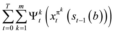
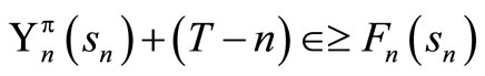
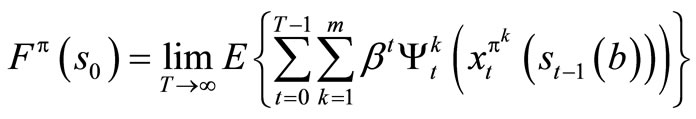
If the profit for allocating the k task to the machines at period t is , the state of the machines is st, number of machines allocated to operate on task k at period t under policy π, is
  and the number of break down machines is bt, then the profit that will accrue to the company over T-horizon is given by
 .
.
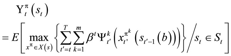
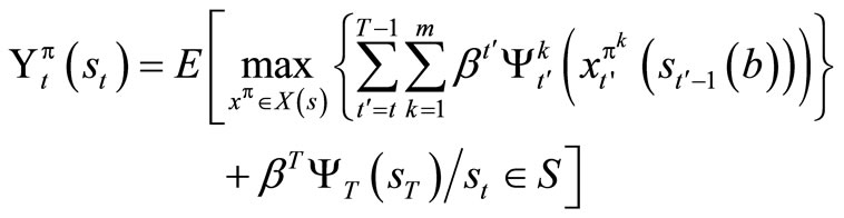
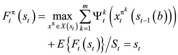
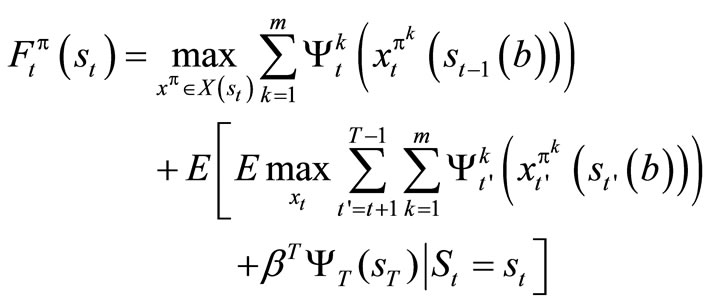
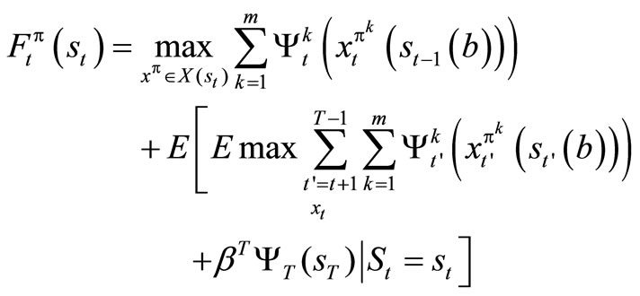
The expected maximum profit that will accrue to the company under policy π is given by
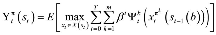 (1)
(1)
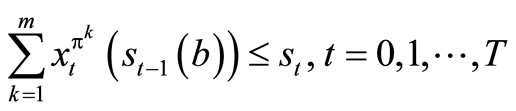
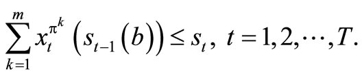
subject to
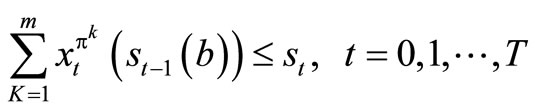 (2)
(2)
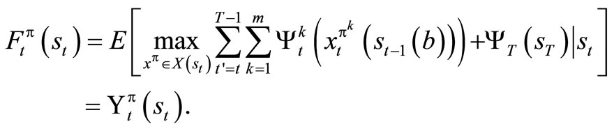
Note: X(st) is the set of possible solution of problem (1). Conditioning (1) on . We now have the following optimization problem (3)
 . (3)
. (3)
Problem (1.3) maximizes the expected profit over X(st) subject to
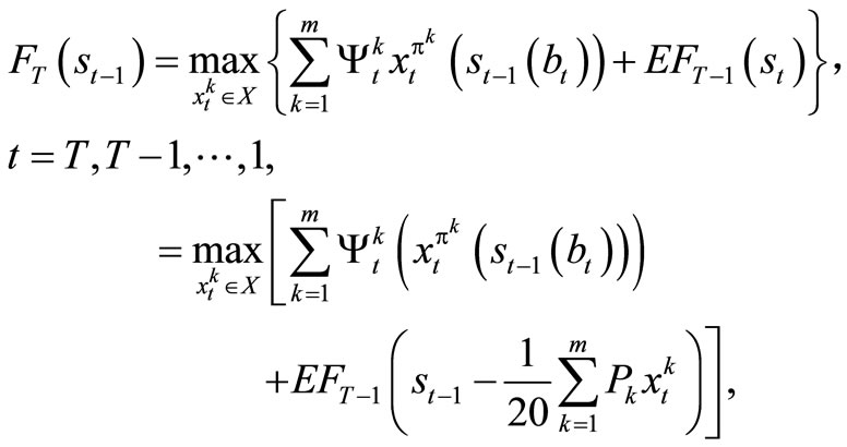
For the profit function , if we accumulate the profit of the first T-stage and add to it the terminal profit
 then (3) becomes
 (4)
(4)
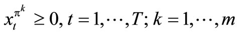
subject to 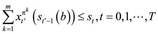 .
.
 .
.
4. Dynamic Programming Formulation and Optimality
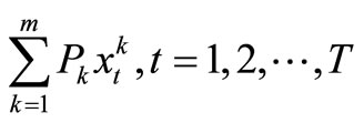
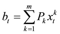
Using st as the state variable at period t and S as the state space, we can formulate the problem as a dynamic program. The number of breakdown machines for task k at period t is given by , where Pk is the probability of break down machines for task k. Hence, total number of break down machines for all the tasks is given by
 .
.
We therefore have that
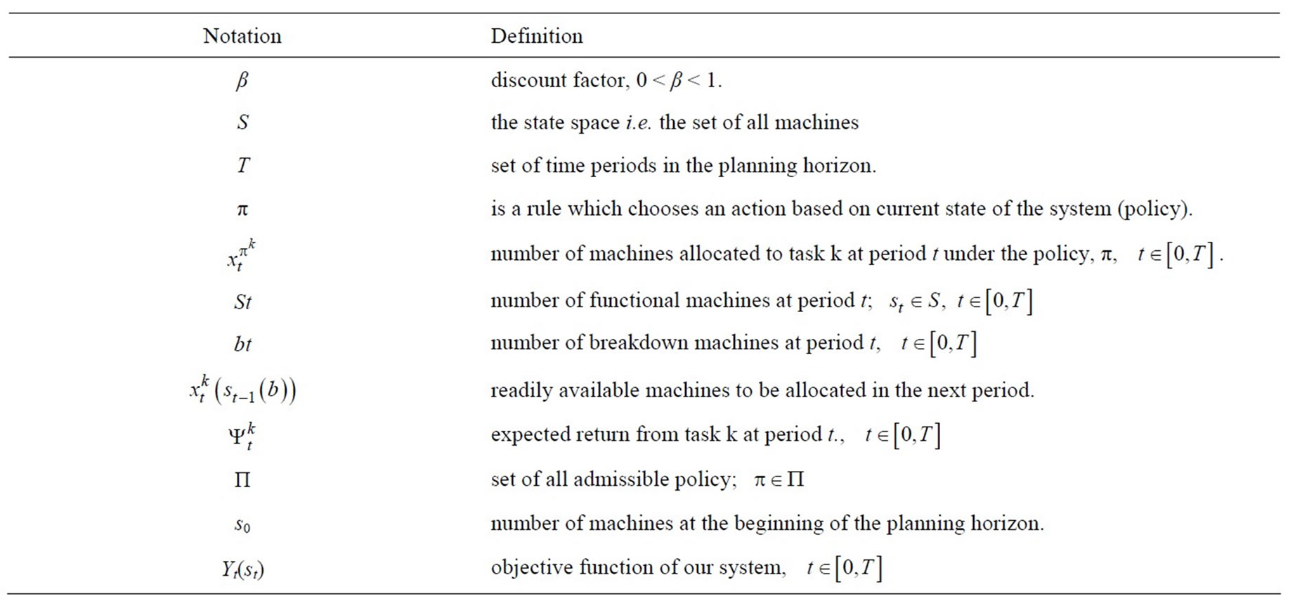
Table 1. Notations and their Definitions.
 .
.
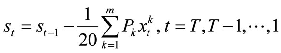
Let st be the number of machines to be allocated in period t and let α be the percentage of break down (but repaired) machines that are expected to join the functional ones in period t, then the transformation equation for the system is given by
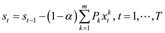 . (5)
. (5)
Observe that the transformation equation is a random variable.
We now set 1 – α = β in (5) to have,
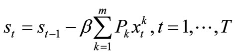 . (6)
. (6)
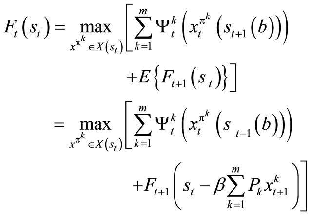
In this case, the optimal policy can be found by computing the value functions through the optimization problem
 (7)
(7)
subject to
Equivalently,
 . (8)
. (8)
 .
.
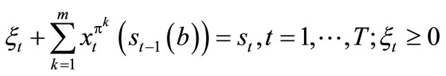
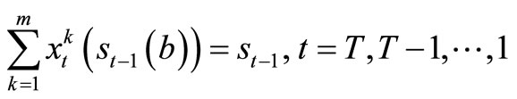
Since all the available functional machines must be allocated in the next period, we have that , for all
 , which is the slack variable.
We show that (4) is equivalent to (7), and then use (4) and (7) interchangeably. The theorem below establish this claim.
Lemma 1.1: Let st be a state variable that captures the relevant history up to time t, and let  be some function measured at t’ ≥ t + 1 conditionalon the random variable st. Then,
 .
.
For the proof, see [3].
Theorem 1.1: Suppose that  satisfies (4) and
  satisfies (7), then
 .
.
Proof: We are to show that . We first use a standard method of DP. Obviously
 .
.
Suppose that it hold for t + 1, t + 2, ···, T, then we show that it is true for t.
We now write
Applying Lemma 1.1, we have
When we condition on , we obtain
For any given objective function, we desire to find the best possible policy, π, that optimizes it, that is, we search for
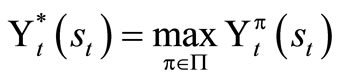 .
.
This is obtained by solving the optimality equation
 (9)
(9)
If we find the set of F’s that solves (9), then we have found the policy that optimizes . The result below establishes this claim.
Theorem 1.2: The expression  is a solution to equation (1.9) if and only if
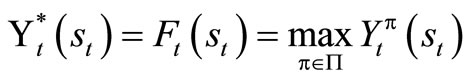 .
.
The if part: This is shows by induction that , for all
 .
.
Since  for all sT and
 , we have that
 .
.
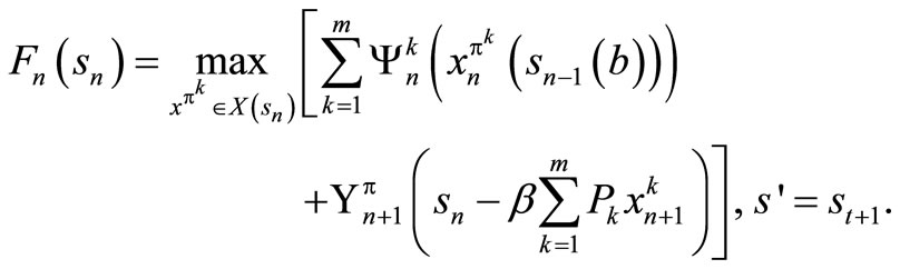
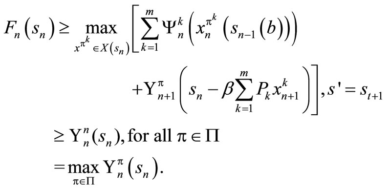
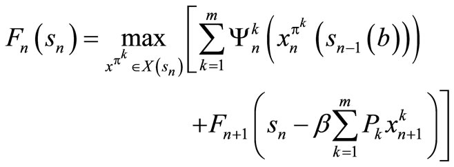
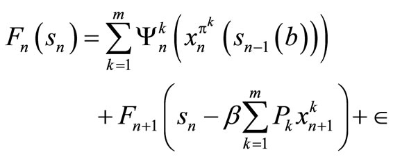
Suppose that , for t = n + 1, n + 2, ···, T, and let
  be an arbitrary policy. For t = n, we obtain the optimality equation as follows
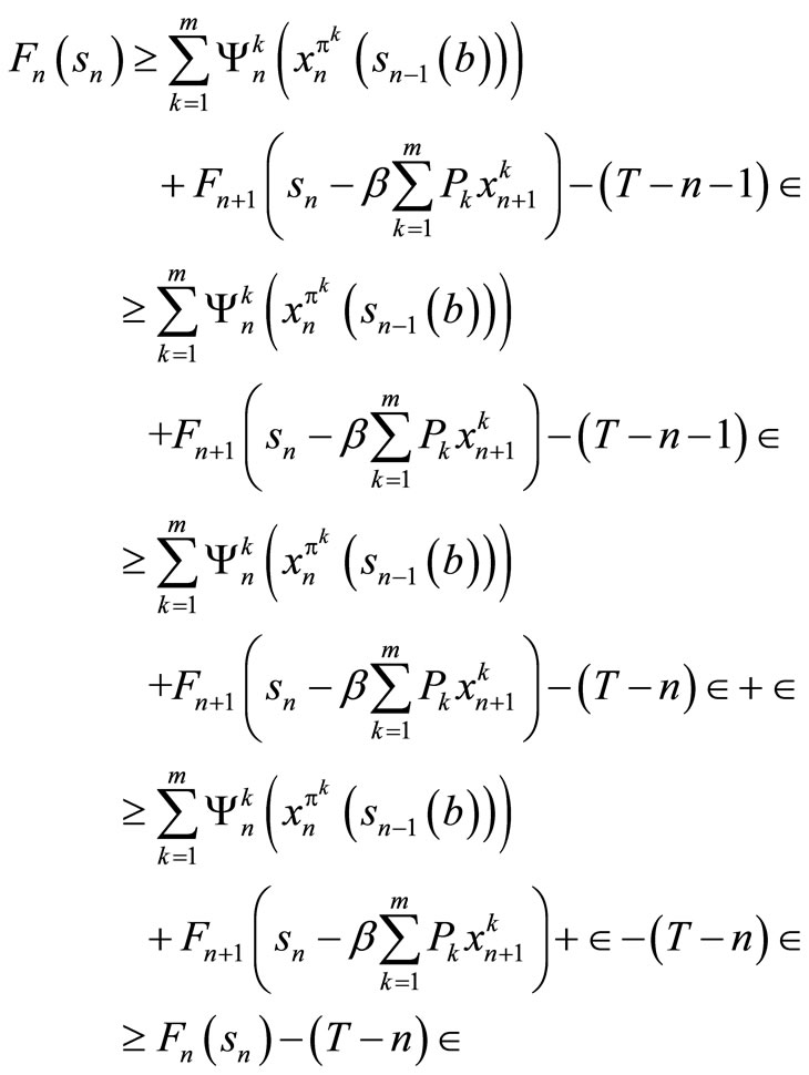
By induction hypothesis,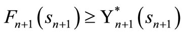 . So we have
Also, we have that 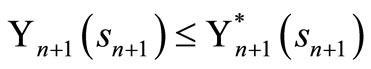 for an arbitrary policy,
  , hence
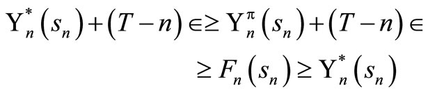
Only if part: We show that for any , there exists
  that satisfies the following:
 (10)
(10)
We now define  as follows:
 (11)
(11)
Let  be the decision rule that solves (1) and satisfies the following:
 (12)
(12)
We now prove (10) by induction. Assume that it is true for t = n + 1, n + 2, ···, T. But,

We now use the induction hypothesis which says
 so that
Hence,
This result shows that solving the optimality equation also gives the optimal value function.
Theorem 1.3: 1) Let B(s) be the set of all bounded real-valued functions F: S → R. The mapping Γ: B(s) → B(s) is a contraction.
2) The operator Γ has a unique fixed point (given by F*).
3) For any F, .
.
4) For any F, if ΓF ≤ F, then F* ≤ ΓtF,
 .
.
Note: Γ is called dynamic programming operator (See [5], for more detail).
Theorem 1.4: For any bounded return or scoring functions F1: S → R and F2: S → R, and for all t = 0, 1, 2, 3, ···, the inequality below holds
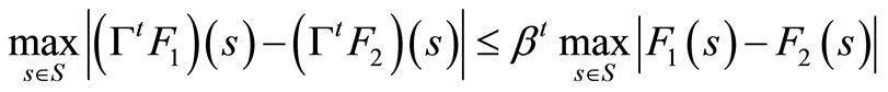
See [8].
The next result shows that as T → ∞, F*(s) → ΓTF(s), . Thus, the profit per stage must be bounded i.e.
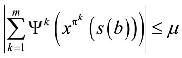 where μ is a positive constant.
We now state this claim formally as follows:
Theorem 1.5: For any bounded return or scoring function F: S → R, FT(s0) → F(s0), T → ∞ that is,
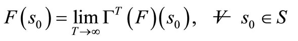 .
.
Proof: Let H be a positive integer,  and policy π = {π0, π1, ···}, we can decompose the return
into the portion received over the first H stages and over the remaining stages.
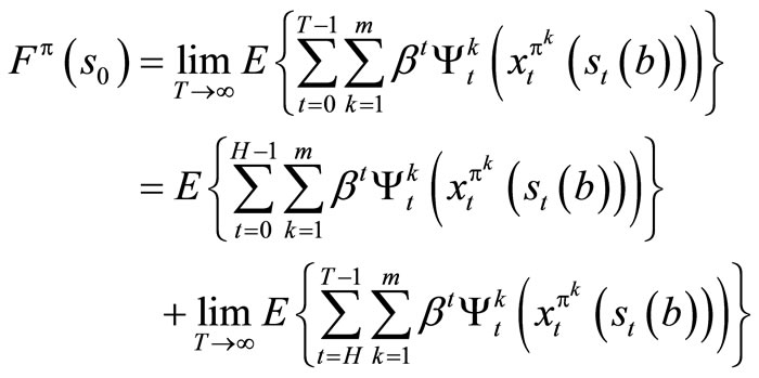
But
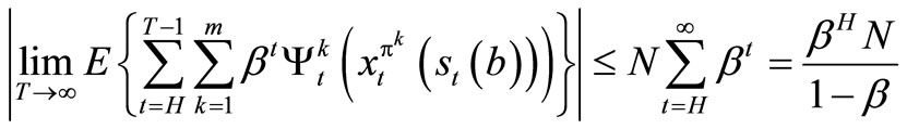
Since 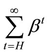
is a geometric progression and 0 < β <1.
Now
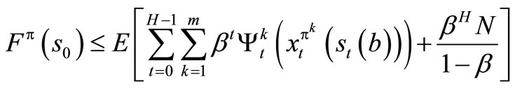
using this relations, it follows that
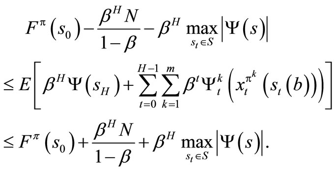
By taking the maximum over π, we obtain for all S0 and H.
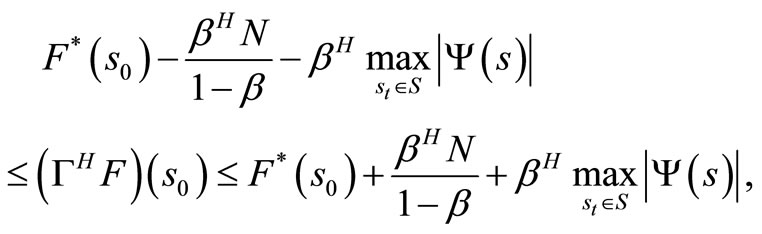
and by taking the unit as H → ∞, we have
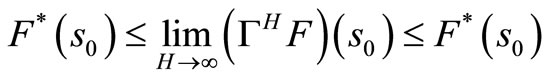
Hence, 
This result shows that our optimization problem converges to a fixed point F* in an infinite horizon.
We use value iteration algorithm for finite and infinite stage to solve our problem. The algorithm converges to an optimal policy.
Step 1: Initialization Set 
Set n = 0 Set 0 < β < 1 Fix a tolerance parameter, ε > 0.
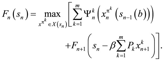
Step 2: For each , calculate
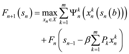 (13)
(13)
Let xn+1 be the decision vector that solve (13).
Step 3: For β = 1:
If 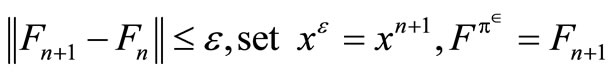 and stop; else set n = n + 1and return to step 2.
Step 4: For 0 < β < 1;
If 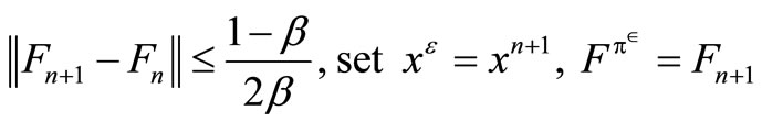
and result stop; else set n = n + 1 and return to step 2.
The theorem below guarantees the convergent of the algorithm.
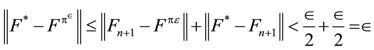
Theorem 1.6: If the algorithm with stopping parameter ε, terminates at iteration n with value function Fn+1, then
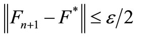 (14)
(14)
In addition, if xε is the optimal decision rule and  is the value of this policy, then
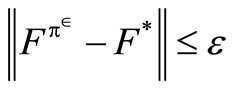 . (15)
This theorem implies that  is the fixed point of the equation F = Γ(xε)F. Since xε is the decision that solves ΓFn+1, it implies that Γ(xε)Fn + 1 = ΓFn+1. Since
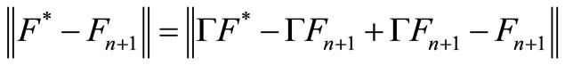 Fn+1 = ΓFn and Γ is contraction, we have that
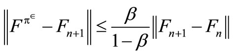
and
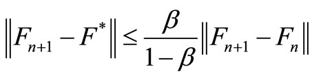 (16)
(16)
But the value iteration algorithm stops when
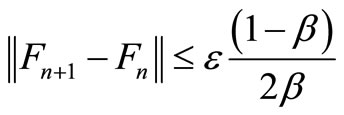 (17)
(17)
From (16) and (17), we have
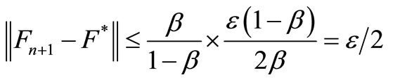 (18)
(18)
Similarly, 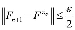
Therefore,
 .
.
5. Computational Result
A production company in Nigeria proposed to purchase 50 machines that can perform nine different tasks. These machines are subject to breakdown. The Table 2 gives information of their decisions.
The company further estimated that out of the number of breakdown machines per week, 95% will join the functional ones for the next period.
The aim of the company is to maximize profit over T horizon Let st represents the number of machines to be allocated in the next period, so that . Since s0 is the number of machines at the beginning of the planning horizon,
is the total number of breakdown machines, and
is expected to join the functional machines in the next period of operation, we have that
 which is our transformation equation and is a random variable.
We can now express our one-period expected return function as follows:
 (19)
(19)
subject to
 .
.
(The feasible region for stage t).
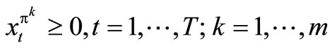
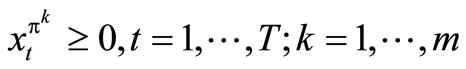
Since the company cannot allocate negative resources to any one task, we write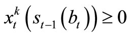 , t = T, T – 1, ···, 1; k = 1, ···, m.
Of course, (19) is the same as
t = T, T – 1, ···, 1, and , t = T, T – 1, ···, 1; k = 1, ···,m.
Note: Our problem has 9 tasks and 48 periods.
Hence, m = 9 and T = 48. Set .
.
Therefore,
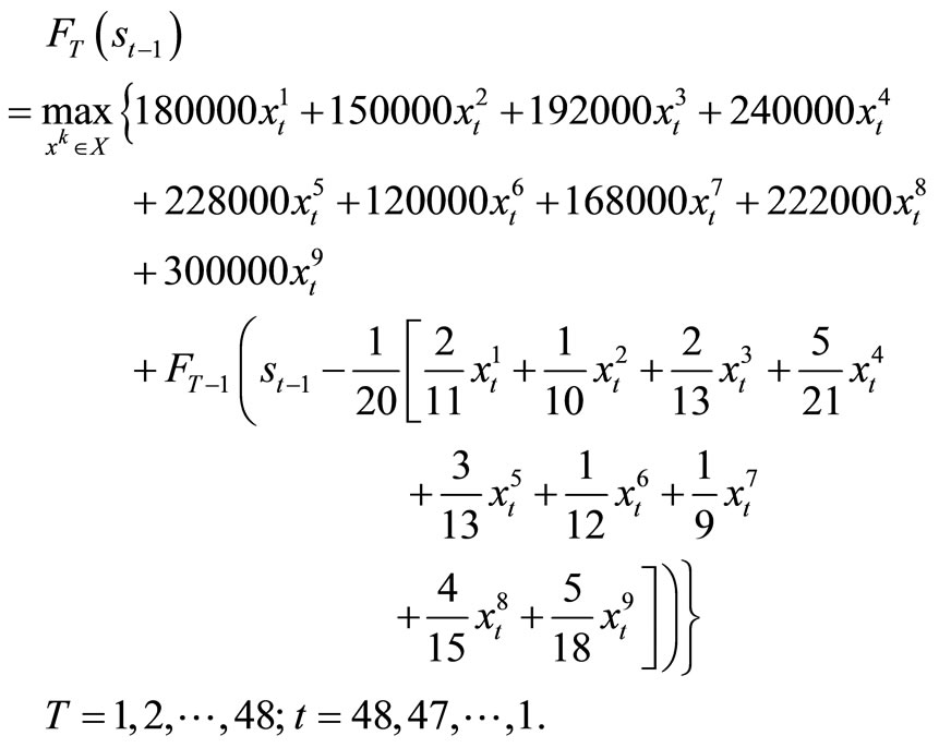 (20)
(20)
subject to:
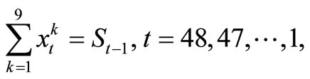
 , t = 48, 47, ···, 1; k = 1, ···, 9 which is a parametric linear programming problem with 9 variables.
A program using MatLab was used for (20). At the end, the following results were obtained.
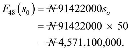
The profit over 48 weeks is given by
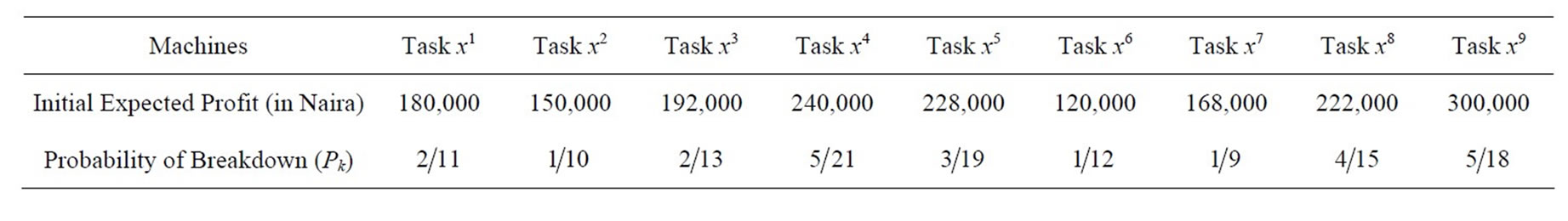
Table 2. The Expected Initial Profit and Probability of Breakdown Machines.
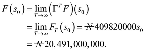
By theorem 1.5, as T approach infinity, FT(s0) approaches F(s0),
and the optimal policy , (t = 1, 2, ···), approaches the limit zero.
Discussion: Figure 1 shows the expected profit that will accrued to the company over a period of 48 weeks. We found that at 48 weeks, the maximum profit that accrued to the company to be 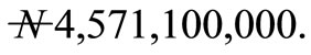 Figure 2 shows the expected profit that will accrued to the
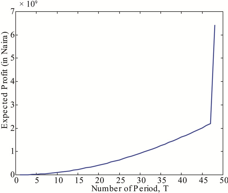
Figure 1. The Expected Profit that will accrued to the Company over a Period of 48 weeks.
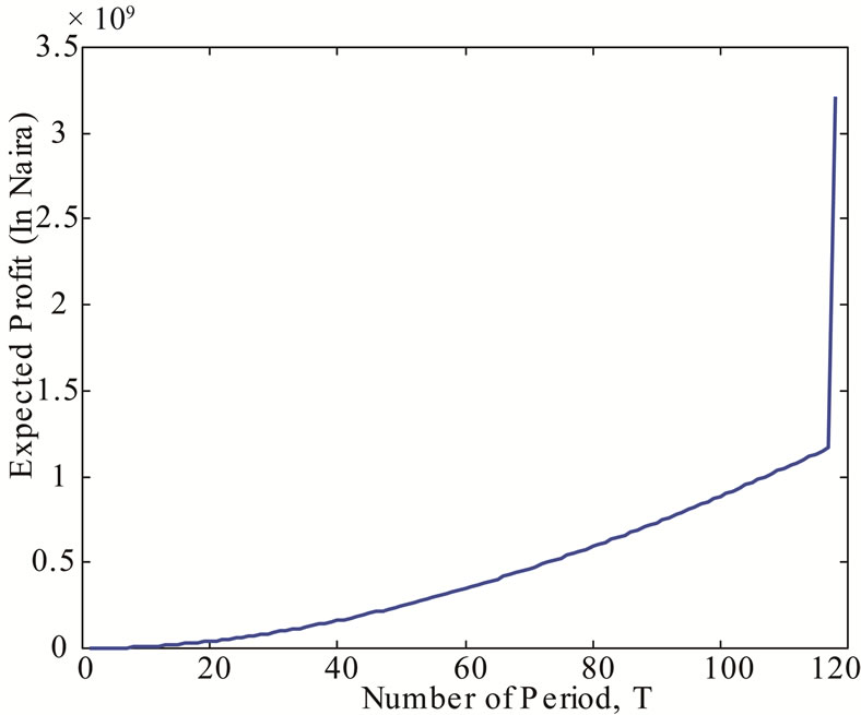
Figure 2. The Expected Profit that will accrued to the Company over an Infinite Period.
company over an infinite weeks. It was found that at infinity, the maximum profit that will accrued to the company to be 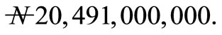
6. Conclusion
Many production companies have for long been allocating resources to different tasks without putting into consideration certain factors that may hinder the realization of their objectives. This paper dealt with allocation of machines to tasks in order to maximize profit over finite and infinite horizon. Careful analysis of the situation reveals that adequate planning, prompt and effective maintainance can enhances the profitability of the company.
REFERENCES
- J. M. Mulvey and H. Vladimirou, “Stochastic Network Programming for Financial Planning Problems,” Management Science, Vol. 38, No. 11, 1992, pp. 1642-1664. doi:10.1287/mnsc.38.11.1642
- B. Van Roy, D. P. Bertsekas, Y. Lee and J. N. Tsitsiklis, “A Neuro-Dynamic Programming Approach to Retailer Inventory Management,” Proceedings of the 36th IEEE Conference on Decision and Control, San Diego, 10-12 December 1997, pp. 4052-4057. doi:10.1109/CDC.1997.652501
- W. B. Powell, “A Comparative Review of Alternative Algorithms for the Dynamic Vehicle Allocation Problem,” In: B. Golden and A. Assad, Eds., Vehicle Routing: Methods and Studies, North Holland, Amsterdam, 1988, pp. 249-292.
- W. B. Powell and H. Topaloglu, “Stochastic Programming in Transportation and Logistics,” In: A. Ruszczynski and A. Shapiro, Eds., Handbook in Operation Research and Management Science, Volume on Stochastic Programming, Elsevier, Amsterdam, 2003, pp. 555-635.
- W. B. Powell, “Approximate Dynamic Programming for Asset Management,” Princeton University, Princeton, 2004.
- H. Topaloglu and S. Kunnumkal, “Approximate Dynamic Programming Methods for an Inventory Allocation Problem under Uncertainty,” Cornell University, Ithaca, 2006.
- C. I. Nkeki, “On A Dynamic Programming Algorithm for Resource Allocation Problems,” Unpublished M.Sc. Thesis, University of Ibadan, Ibadan, 2006.
- D. P. Bertsekas, “Dynamic Programming and Optimal Control,” 2nd Edition, Vol. 2, Athena Scientific, Belmont, 2001.