American Journal of Operations Research
Vol. 2 No. 1 (2012) , Article ID: 17836 , 6 pages DOI:10.4236/ajor.2012.21011
Optimizing Forest Sampling by Using Lagrange Multipliers
Department of Forestry and Management of the Environment and Natural Resources, Democritus University of Thrace, Orestiada, Greece
Email: kkitikid@fmenr.duth.gr
Received July 22, 2011; revised August 20, 2011; accepted September 10, 2011
Keywords: Forest Inventories; Lagrange Multipliers; Optimization, Sampling
ABSTRACT
In two-phase sampling, or double sampling, from a population with size N we take one, relatively large, sample size n. From this relatively large sample we take a small sub-sample size m, which usually costs more per sample unit than the first one. In double sampling with regression estimators, the sample of the first phase n is used for the estimation of the average of an auxiliary variable X, which should be strongly related to the main variable Y (which is estimated from the sub-sample m). Sampling optimization can be achieved by minimizing cost C with fixed , or by finding a minimum
  for fixed C. In this paper we optimize sampling with use of Lagrange multipliers, either by minimizing variance of Y and having predetermined cost, or by minimizing cost and having predetermined variance of Y.
1. Introduction
All decision-making requires information. In forestry, this information is acquired by means of forest inventories, systems for measuring the extent, quantity and condition of forests [1]. More specifically, the purpose of forest inventories is to estimate means and totals for measures of forest characteristics over a defined area. Such characteristics include the volume of the growing stock, the area of a certain type of forest and nowadays also measures concerned with forest biodiversity, e.g. the volume of dead wood or vegetation.
The main method used in forest inventories in the 19th century was complete enumeration, but it was soon noted that there was a possibility to reduce costs by using representative samples [2]. Sampling-based methods were used in forestry a century before the mathematical foundations of sampling techniques were described [3-9]. In this paper we attempt to optimize sampling with use of Lagrange multipliers, either by minimizing variance of the forest variable we are interested in and having fixed cost, or by minimizing cost and having fixed variance of the variable in question.
2. The Method of Lagrange Multipliers
Lagrange multipliers is a method of evaluating maxima or minima of a function of possibly several variables, subject to one or more constraints [10]. This method, which is due to Joseph Louis de Lagrange (1736-1813), is used to optimize a real-valued function , where x1, x2,
  , xn are subject to m (<n) equality constraints of the form
 (1)
(1)
where g1, g2,  , gn are differentiable functions.
This determination of the stationary points in this constrained optimization problem is done by first considering the function
 (2)
(2)
where  and λ1, λ2,
  , λm are scalars called Lagrange multipliers. By differentiating (2) with respect to x1, x2,
  , xn and equating the partial derivatives to zero we obtain
 (3)
(3)
Equations (1) and (3) consist of m + n unknowns, namely, x1, x2,  , xn; λ1, λ2,
  , λm. The solutions for x1, x2,
  , xn determine the locations of the stationary points. The following argument explains why this is the case.
Suppose that in Equation (1) we can solve for m xi’s, for example, x1, x2,  , xn, in terms of the remaining n – m variables. By Implicit Function Theorem (see Appendix 1), this is possible whenever
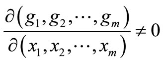 . (4)
. (4)
In this case, we can write
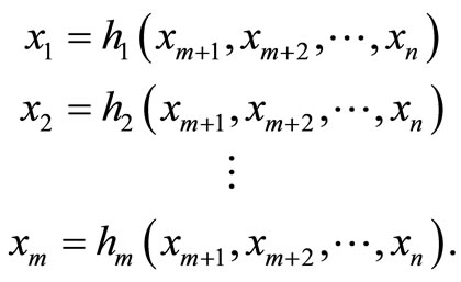 (5)
(5)
Thus f(x) is a function of only n – m variables, namely, xm+1, xm+2,  , xn. If the partial derivatives of f with respect to these variables exist and if f has a local optimum, then these partial derivatives must necessarily vanish, that is,
 (6)
(6)
Now, if Equations (5) are used to substitute h1, h2,  , hm for x1, x2,
  , xn, respectively, in Equation (1), then we obtain the identities
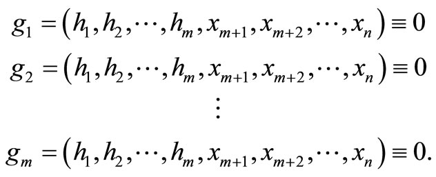 .
.
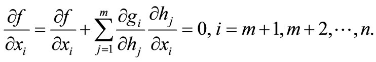
By differentiating these identities with respect to xm+1, xm+2,  , xn we obtain
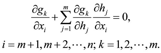 (7)
(7)
Let us now define the vectors
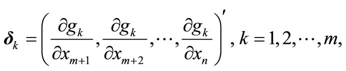

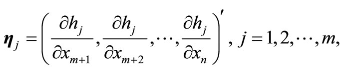
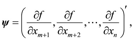
 .
.
Equations (6) and (7) can then be written as
 (8)
(8)
 (9)
(9)
where , which is a nonsingular m × m matrix if condition (4) is valid.
From Equation (8) we have

By making the proper substitution in Equation (9) we obtain
 , (10)
where
 . (11)
Equations (10) can then be expressed as
 (12)
(12)
From Equation (11) we also have
 (13)
(13)
Equations (12) and (13) can now be combined into a single vector equation of the form
 which is the same as Equation (3). We conclude that at a stationary point of f, the values of x1, x2,
  , xn and the corresponding values of λ1, λ2,
  , λm must satisfy Equations (1) and (3).
3. Lagrange Multipliers in Sampling Optimization
In two-phase sampling, or double sampling, from a population with size N we take one, relatively large, sample size n. From this relatively large sample we take a small sub-sample size m, which usually costs more per sample unit than the first one. In double sampling with regression estimators, the sample of the first phase n is used for the estimation of the average of an auxiliary variable X,  , which should be strongly related to the main variable Y.
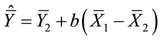
In the sub-sample m both auxiliary X and main Y variables are measured, in order to estimate their means 
and , respectively. The regression estimator
  and its estimated variance
  are ([7,11-13]):
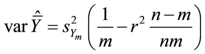
where  is the variance of Y in the sub-sample m, and r is the estimated correlation coefficient between X and Y.
An approximate cost function could be
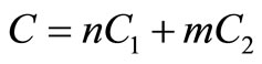 where C: total sampling cost;
C1: sampling cost of the first phase;
C2: sampling cost of the second phase.
Sampling optimization can be achieved by minimizing cost C with fixed , applying the following procedure:
We assume an approximately normal distribution of , so that the 95% confidence interval for
  would be:
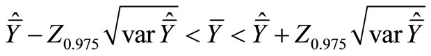 where
where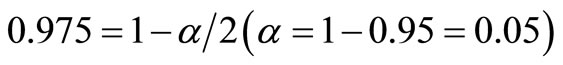 .
.
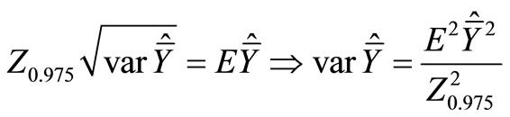
Now we must choose n and m in such a way, that half a confidence interval does not exceed a value D, fixed a priori, where D also may be expressed as a fraction (E)
of :
:
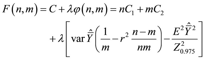
To this end we construct the Lagrange function:
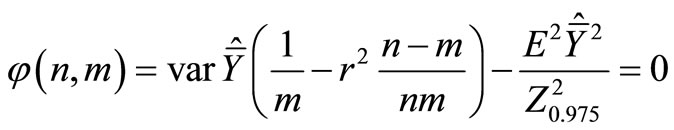
Remind that
 so
so
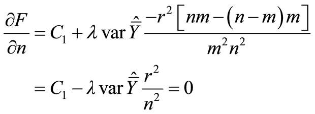 (14)
(14)
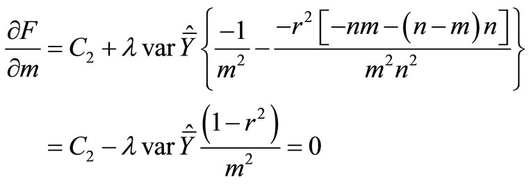 (15)
(15)
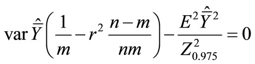 (16)
(16)
Solving the system of Equations (14), (15) and (16) we find n, m and λ. The reverse problem, viz. finding  for fixed C, is solved in a similar way.
In order to explain how Lagrange multipliers work, we describe the following example: Assume that the total cost C of an industry producing two products x and y, is given by the equation . The production is limited with a limitation of 20 units, that is
 . Thus, we have:

 (a)
(a)
 (b)
(b)
 (c)
(c)
By solving the equations’ system (a), (b) and (c), we find that x = 13, y = 7 and λ = –71. Consequently, .
.
The economic meaning of λ is this: λ is the reduction of the total cost to the limit, if production was 19 instead of 20 units. In other words, if we required 19 total production units, the total cost would be reduced by 71 monetary units (710 – 71 = 639). Generally, λ represents the marginal effect on the cost function, when production limitation is increased by one unit.
4. Other Uses of Lagrange Multipliers in Forest Inventories
If there are not enough sample plots to give sufficiently good inventory results using only forest measurements, we may try to make use of auxiliary variables correlated with forest variables. The most obvious way is to use ratio or regression estimators (see Appendix 2). The calibration estimator of Deville and Särndal [14] is an extension of the regression estimator for obtaining population totals using auxiliary information. Both regression and calibration estimators can be employed if there are auxiliary variables for inventory sample plots known for which the population totals are also known, e.g. variables obtained from remote sensing or from GIS systems. The appeal of calibration estimators for forest inventories comes from the fact that they lead to estimators which are weighted sums of the sample plot variables, where the weight can be interpreted as the area of forest in the population that is similar to the sample plot.
The basic features of the calibration estimator of Deville and Särndal [14] in terms of estimating means can be described as follows. Consider a finite population U consisting of N units. Let j denote a general unit, thus . In a forest inventory the population is a region where units are pixels or potential sample plots. The units in a forest inventory will be referred to here as pixels, and it will be assumed that an inventory sample plot gives values to the forest variables for an associated pixel. Each unit j is associated with a variable yj and a vector of auxiliary variables xj. The population mean of x,
  is assumed to be known. The y variables in a forest inventory are forest variables and the x variables can be spectral variables from remote sensing or geographical or climatic variables obtained from GIS databases.
Assume that a probability sample S is drawn, and yj and xj are observed for each j in S, the objective being to estimate the mean of y, . Let πj be the inclusion probability and dj the basic sampling design weight
 , which can be used to compute the unbiased Horvitz-Thompson estimator
 .
.
A calibration estimator
 (17)
(17)
is obtained by minimizing the sum of distances,
 , between the prior weights dj and posterior weights wj for a positive distance function G, taking account of the calibration equation
 . (18)
If the distance between dj and wj is defined as
 the calibration estimator will be the same as the regression estimator
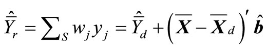 , (19)
where  and
and  (a weighted regression coefficient vector) are
 (20)
(20)
and
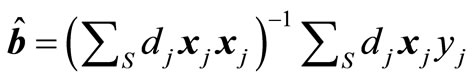 . (21)
If the model contains an intercept, the corresponding variable x will be one for all observations, and the calibration Equation (18) will then guarantee that the weights wj add up to one. This means that when estimating totals, the weights Nwj will add up to the known total number of pixels in the population. Thus Nwj can be interpreted as the total area, in pixel units, for plots of forest similar to plot j. The standard least squares theory implies that the regression estimator (19) can be expressed in the form
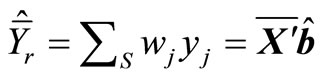 . (22)
It is assumed that the intercept is always among the parameters. Estimator (21) is defined if the moment matrix 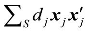 is non-singular.
Some of the weights wj in (17) implied by Equations (20)-(22) may be negative. Nonnegative weights are guaranteed if the distance function is infinite for negative wj. Deville and Särndal [14] presented four distance functions producing positive weights.
Minimization of the sum , so that (18) is satisfied is a non-linear constrained minimization problem. Using Lagrange multipliers, the problem can be reformulated as a non-linear system of equations which can be solved iteratively using Newton’s method [14]. If the initial values of the Lagrange multipliers are set to zero, the first step will produce wj’s of the regression estimator (19).
Since the calibration estimator is asymptotically equivalent to the regression estimator, Deville and Särndal [14] suggest that the variance of the calibration estimator should be computed in the same way as the variance of the regression estimator using regression residuals. There is no design-unbiased estimator of the variance in systematic sampling [7].
The emphasis on area interpretation for the weights has the same argument behind it as was used by Moeur and Stage [14] for the most similar neighbour method (MSN), where unknown plot variables are taken from a plot which is as similar as possible with respect to the known plot variables. In both methods each sample plot represents a percentage of the total area, and all the forest variables are logically related to each other. The difference is that in the calibration estimator we obtain an estimate of the area of the sample plot for the whole population whereas in the MSN method each pixel is associated with a sample plot. Since there is no straightforward way of showing that the MSN method produces optimal results in any way at the population level, it may be safer to use the calibration estimator for computing population-level estimates for forest variables. The problem with the calibration estimator is that it does not provide a map. If a map is needed, then the weights provided by the calibration estimator need to be distributed over pixels using separate after-processing.
Lappi [15] proposed a small-area modification of the calibration estimator which can be used when several subpopulation totals are required simultaneously. He used satellite data as auxiliary information for computing inventory results for counties. Sample plots in the surrounding inclusion zone are also used for a given subpopulation so that the prior weight decreases as distance increases. The error variance is computed using a spatial variogram model. Block kriging [16] provides an optimal estimator for subpopulation totals under such a model, but kriging can produce negative weights for sample plots, and the weights are different for each y variable. Thus it is not possible to give areal interpretations to sample plot weights in kriging.
REFERENCES
- J. Penman, M. Gytarsky, T. Hiraishi, T. Krug, D. Kruger, R. Pipatti, L. Buendia, K. Miwa, T. Ngara, K. Tanabe and F. Wagner, “Good Practice Guidance for Land Use, LandUse Change and Forestry,” Intergovernmental Panel on Climate Change: IPCC National Greenhouse Gas Inventories Program, Institute for Global Environmental Strategies (IGES) for the IPCC, Kanagawa Japan, 2003.
- F. Loetsch, F. Zöhrer and K. Haller, “Forest Inventory,” BLV, Verlagsgesellschaft, 1973.
- I. Doig, “When the Douglas-Firs Were Counted: The Beginning of the Forest Survey,” Journal of Forest History, Vol. 20, 1976, pp. 20-27.
- W. Frayer and G. Furnival, “Forest Survey Sampling Designs—A History,” Journal of Forestry, Vol. 97, No. 12, 1999, pp. 4-10.
- T. Gregoire, “Roots of Forest Inventory in North America,” A Paper Presented at the A1 Inventory Working Group Session at the SAF National Convention Held at Richmond, VA, 25-28 October 1992.
- T. Honer and F. Hegyi, “Forest Inventory—Growth and Yield in Canada: Past, Present and Future,” The Forestry Chronicle, Vol. 66, 1990, pp. 112-117.
- H. Schreuder, T. Gregoire and G. Wood, “Sampling Methods for Multiresource Forest Inventory,” John Wiley and Sons, New York, 1993.
- R. Seppälä, “Forest Inventories and the Development of Sampling Methods,” Silva Fennica, Vol. 3, 1985, pp. 218-219.
- D. Van Hooser, N. Cost and H. Lund, “The History of Forest Survey Program in the United States,” In: G. Preto and B. Koch, Eds., Forest Resource Inventory and Monitoring and Remote Sensing Technology, Proceedings of the IUFRO Centennial Meeting in Berlin, 31 August-4 September 1992, Japan Society of Forest Planning Press, Tokyo University of Agriculture and Technology, Saiwaicho, Fuchu, Tokyo, 1992, pp. 19-27.
- S. Rao, “Optimization Theory and Application,” Wiley Eastern Ltd., New Delhi, 1984.
- W. Cochran, “Sampling Techniques—3rd Edition,” Wiley, New York, 1977.
- P. De Vries, “Sampling for Forest Inventory,” Springer, Berlin, 1986. doi:10.1007/978-3-642-71581-5
- K. Matis, “Sampling of Natural Resources,” Pigasos Publications, Thessaloniki, Greece, 2004.
- J. Deville and C. Särndal, “Calibration Estimators in Survey Sampling,” Journal of the American Statistical Association, Vol. 87, No. 418, 1992, pp. 376-382. doi:10.2307/2290268
- J. Lappi, “Forest Inventory of Small Areas Combining the Calibration Estimator and a Spatial Model,” Canadian Journal of Forest Research, Vol. 31, No. 9, 2001, pp. 1551-1560. doi:10.1139/x01-078
- N. Cressie, “Kriging Nonstationary Data,” Journal of American Statistical Association, Vol. 81, No. 395, 1986, pp. 625-634. doi:10.2307/2288990
- M. Moeur and A. Stage, “Most Similar Neighbor: An Improved Sampling Inference Procedure for Natural Resource Planning,” Forest Science, Vol. 41, No. 2, 1995, pp. 337-359.
Appendices
Appendix 1. Implicit Function Theorem
Let , where D is an open subset of Rm + n, and g has continuous first-order partial derivatives in D. If there is a point
 , where
 , with
 ,
,  such that
 , and if at z0,
 where gi is the ith element of
 , then there is a neighborhood
  of y0 in which the equation
  can be solved uniquely for x as a continuously differentiable function of y.
Appendix 2. Ratio and Regression Estimators
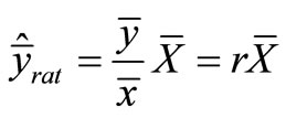
In a stratified inventory information on some auxiliary variables is used both to plan the sampling design (e.g. allocation) and for estimation, or only for estimation (post-stratification). Stratification is not the only way to use auxiliary information, however, as it can be used at the design stage, e.g. in sampling proportional to size (see Appendix 3). It can also be used at the estimation stage in ratio or regression estimators, so that the standard error of the estimators can be reduced using information on a variable x which is known for each sampling unit in the population. The estimation is based on the relationship between the variables x and y. In ratio estimation, a model that goes through the origin is applied. If this model does not apply, regression estimator is more suitable. The ratio estimator for the mean is
 where
where  is the mean of a variable x in the population and
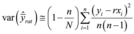
  in the sample. Ratio estimators are usually biased, and thus the root mean square error (RMSE) should be used instead of the standard error. The relative bias nevertheless decreases as a function of sample size, so that in large samples (at least more than 30 units) the accuracy of the mean estimator can be approximated as [1]:
 .
.
The ratio estimator is more efficient the larger the correlation between x and y relative to the ratio of the coefficients of variation CV. It is worthwhile using the ratio estimator if
 .
.
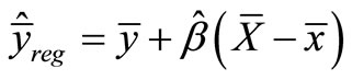
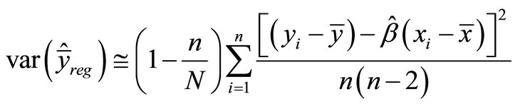
The (simple linear) regression estimator for the mean value is
 where
where  is the OLS (Ordinary Least Squares) coefficient of x for the model, which predicts the population mean of y based on the sample means. In a sampling context, the constant of the model is not usually presented, but the formula for the constant,
 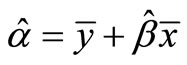 , is embedded in the equation. The model is more efficient the larger the correlation between x and y. The variance of the regression estimator can be estimated as
 .
.
Appendix 3. Sampling with Probability Proportional to Size
The basic properties of sampling with arbitrary probabilities can also be utilized in sampling with probability proportional to size (PPS), such as sampling with a relascope. It is then assumed that unit i is selected with the probability kxi, where k is a constant and x is a covariate (diameter of a tree in relascope sampling). PPS sampling is more efficient the larger the correlation between x and y. For perfect correlation the variance in the estimator would be zero [7]. PPS sampling might even be less efficient than SRS (Simple Random Sampling), however, if the correlation were negative. This could be the case when multiple variables of interest are considered simultaneously, for example, when correlation with one variable (say volume) might give efficient estimates but the estimates for other variables (say health and quality) might not be so good.
In practice, PPS sampling can be performed by ordering the units, calculating the sum of their sizes (say ), and calculating
 . The probability of a unit i being selected is then
  and a cumulative probability can be calculated for the ordered units. A random number r is then picked and each unit with a cumulative probability equal to (or just above) r, r + 1, r + 2,
  , r + n – 1 is selected for the sample. Every unit of size greater than
  is then selected with certainty.