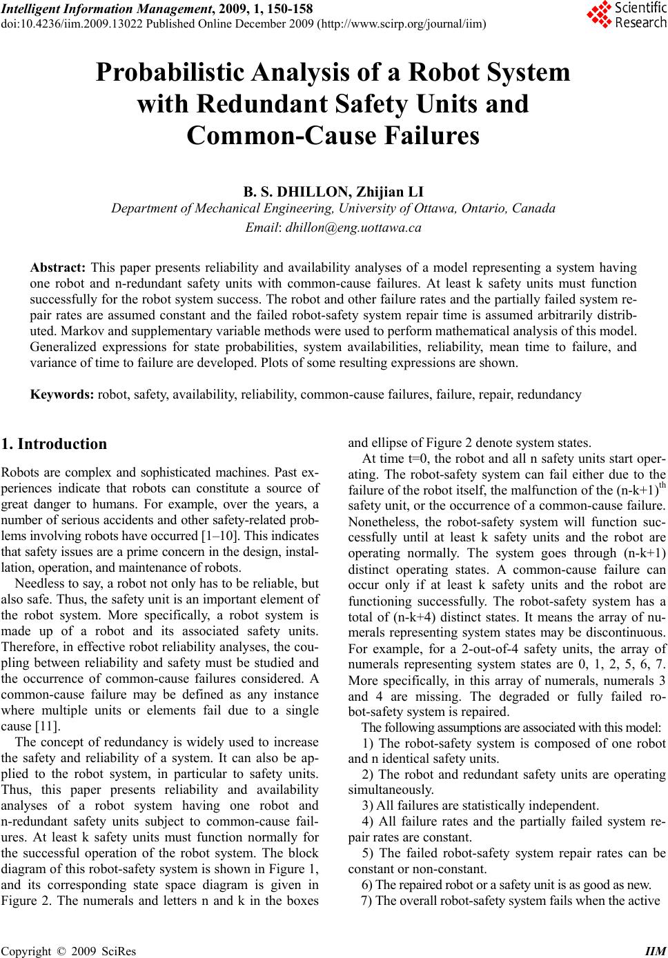Intelligent Information Management, 2009, 1, 150-158
doi:10.4236/iim.2009.13022 Published Online December 2009 (http://www.scirp.org/journal/iim)
Probabilistic Analysis of a Robot System
with Redundant Safety Units and
Common-Cause Failures
B. S. DHILLON, Zhijian LI
Department of Mechanical Engineering, University of Ottawa, Ontario, Canada
Abstract: This paper presents reliability and availability analyses of a model representing a system having
one robot and n-redundant safety units with common-cause failures. At least k safety units must function
successfully for the robot system success. The robot and other failure rates and the partially failed system re-
pair rates are assumed constant and the failed robot-safety system repair time is assumed arbitrarily distrib-
uted. Markov and supplementary variable methods were used to perform mathematical analysis of this model.
Generalized expressions for state probabilities, system availabilities, reliability, mean time to failure, and
variance of time to failure are developed. Plots of some resulting expressions are shown.
Keywords: robot, safety, availability, reliability, common-cause failures, failure, repair, redundancy
1. Introduction
Robots are complex and sophisticated machines. Past ex-
periences indicate that robots can constitute a source of
great danger to humans. For example, over the years, a
number of serious accidents and other safety-related prob-
lems involving robots have occurred [1–10]. This indicates
that safety issues are a prime concern in the design, instal-
lation, operation, and maintenance of robots.
Needless to say, a robot not only has to be reliable, but
also safe. Thus, the safety unit is an important element of
the robot system. More specifically, a robot system is
made up of a robot and its associated safety units.
Therefore, in effective robot reliability analyses, the cou-
pling between reliability and safety must be studied and
the occurrence of common-cause failures considered. A
common-cause failure may be defined as any instance
where multiple units or elements fail due to a single
cause [11].
The concept of redundancy is widely used to increase
the safety and reliability of a system. It can also be ap-
plied to the robot system, in particular to safety units.
Thus, this paper presents reliability and availability
analyses of a robot system having one robot and
n-redundant safety units subject to common-cause fail-
ures. At least k safety units must function normally for
the successful operation of the robot system. The block
diagram of this robot-safety system is shown in Figure 1,
and its corresponding state space diagram is given in
Figure 2. The numerals and letters n and k in the boxes
and ellipse of Figure 2 denote system states.
At time t=0, the robot and all n safety units start oper-
ating. The robot-safety system can fail either due to the
failure of the robot itself, the malfunction of the (n-k+1)th
safety unit, or the occurrence of a common-cause failure.
Nonetheless, the robot-safety system will function suc-
cessfully until at least k safety units and the robot are
operating normally. The system goes through (n-k+1)
distinct operating states. A common-cause failure can
occur only if at least k safety units and the robot are
functioning successfully. The robot-safety system has a
total of (n-k+4) distinct states. It means the array of nu-
merals representing system states may be discontinuous.
For example, for a 2-out-of-4 safety units, the array of
numerals representing system states are 0, 1, 2, 5, 6, 7.
More specifically, in this array of numerals, numerals 3
and 4 are missing. The degraded or fully failed ro-
bot-safety system is repaired.
The following assumptions are associated with this model:
1) The robot-safety system is composed of one robot
and n identical safety units.
2) The robot and redundant safety units are operating
simultaneously.
3) All failures are statistically independent.
4) All failure rates and the partially failed system re-
pair rates are constant.
5) The failed robot-safety system repair rates can be
constant or non-constant.
6) The repaired robot or a safety unit is as good as new.
7) The overall robot-safety system fails when the active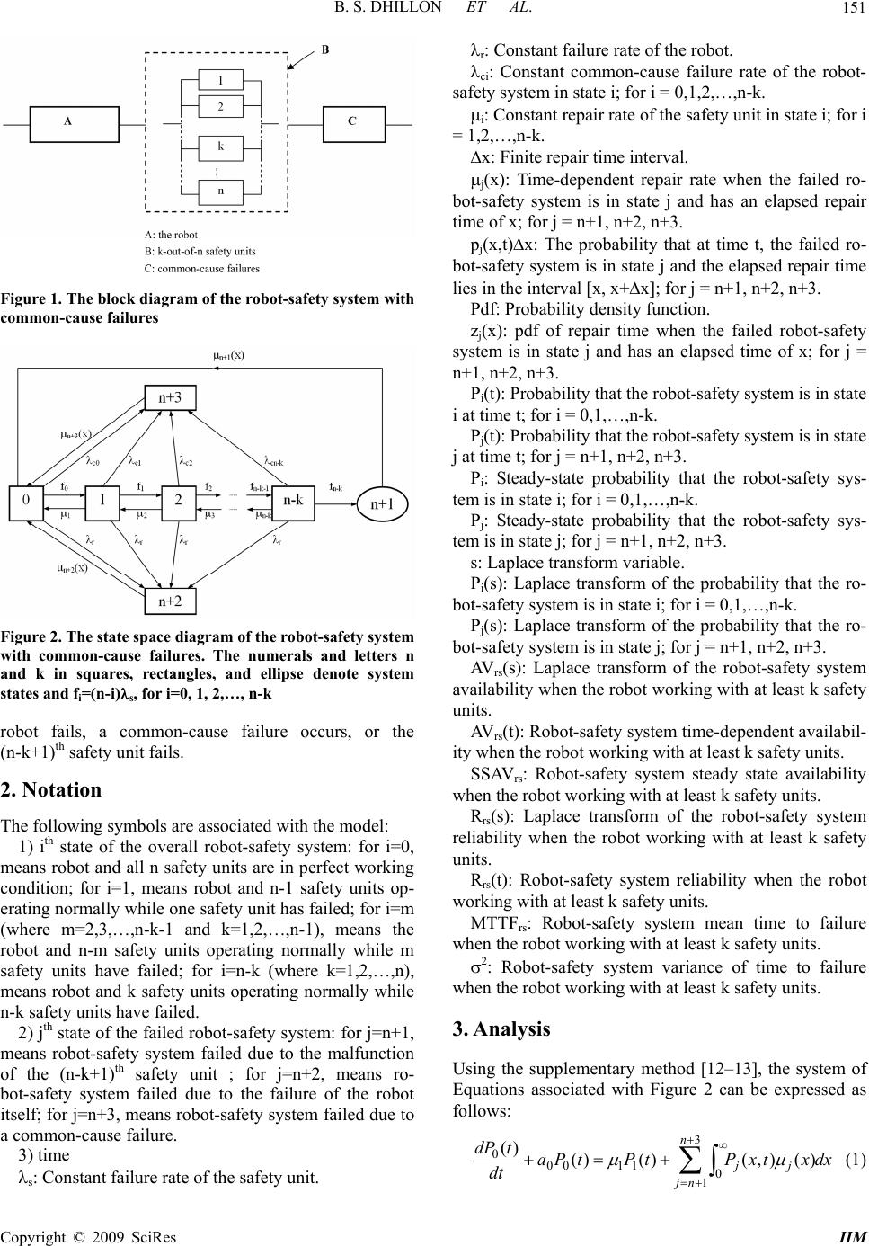

B. S. DHILLON ET AL. 151
Figure 1. The block diagram of the robot-safety system with
common-cause failures
Figure 2. The state space diagram of the robot-safety system
with common-cause failures. The numerals and letters n
and k in squares, rectangles, and ellipse denote system
states and fi=(n-i)s, for i=0, 1, 2,…, n-k
robot fails, a common-cause failure occurs, or the
(n-k+1)th safety unit fails.
2. Notation
The following symbols are associated with the model:
1) ith state of the overall robot-safety system: for i=0,
means robot and all n safety units are in perfect working
condition; for i=1, means robot and n-1 safety units op-
erating normally while one safety unit has failed; for i=m
(where m=2,3,…,n-k-1 and k=1,2,…,n-1), means the
robot and n-m safety units operating normally while m
safety units have failed; for i=n-k (where k=1,2,…,n),
means robot and k safety units operating normally while
n-k safety units have failed.
2) jth state of the failed robot-safety system: for j=n+1,
means robot-safety system failed due to the malfunction
of the (n-k+1)th safety unit ; for j=n+2, means ro-
bot-safety system failed due to the failure of the robot
itself; for j=n+3, means robot-safety system failed due to
a common-cause failure.
3) time
s: Constant failure rate of the safety unit.
r: Constant failure rate of the robot.
ci: Constant common-cause failure rate of the robot-
safety system in state i; for i = 0,1,2,…,n-k.
i: Constant repair rate of the safety unit in state i; for i
= 1,2,…,n-k.
x: Finite repair time interval.
j(x): Time-dependent repair rate when the failed ro-
bot-safety system is in state j and has an elapsed repair
time of x; for j = n+1, n+2, n+3.
pj(x,t)x: The probability that at time t, the failed ro-
bot-safety system is in state j and the elapsed repair time
lies in the interval [x, x+x]; for j = n+1, n+2, n+3.
Pdf: Probability density function.
zj(x): pdf of repair time when the failed robot-safety
system is in state j and has an elapsed time of x; for j =
n+1, n+2, n+3.
Pi(t): Probability that the robot-safety system is in state
i at time t; for i = 0,1,…,n-k.
Pj(t): Probability that the robot-safety system is in state
j at time t; for j = n+1, n+2, n+3.
Pi: Steady-state probability that the robot-safety sys-
tem is in state i; for i = 0,1,…,n-k.
Pj: Steady-state probability that the robot-safety sys-
tem is in state j; for j = n+1, n+2, n+3.
s: Laplace transform variable.
Pi(s): Laplace transform of the probability that the ro-
bot-safety system is in state i; for i = 0,1,…,n-k.
Pj(s): Laplace transform of the probability that the ro-
bot-safety system is in state j; for j = n+1, n+2, n+3.
AV rs(s): Laplace transform of the robot-safety system
availability when the robot working with at least k safety
units.
AV rs(t): Robot-safety system time-dependent availabil-
ity when the robot working with at least k safety units.
SSAVrs: Robot-safety system steady state availability
when the robot working with at least k safety units.
Rrs(s): Laplace transform of the robot-safety system
reliability when the robot working with at least k safety
units.
Rrs(t): Robot-safety system reliability when the robot
working with at least k safety units.
MTTFrs: Robot-safety system mean time to failure
when the robot working with at least k safety units.
2: Robot-safety system variance of time to failure
when the robot working with at least k safety units.
3. Analysis
Using the supplementary method [12–13], the system of
Equations associated with Figure 2 can be expressed as
follows:
dxxtxPtPtPa
dt
tdP n
nj
jj





3
10
1100
0)(),()()(
)(
 (1)

B. S. DHILLON ET AL. 152
)1,...,2,1(
)()()1()(
)(
111

 
knifor
tPtPintPa
dt
tdP
iiisii
i

(2)
)()1()(
)( tPktPa
dt
tdP
knsknkn
kn  
 (3)
0),()(
),(),( 




txPx
x
txP
t
txP
jj
jj
 (4)
)3,2,1(  nnnjfor
where
00 crs
na




)1,...,2,1()(


 kniforina icirsi




knkcnrskn ka  






The associated boundary conditions are as follows:
)(),0(
1tPktPknsn 

(5)




kn
i
irn tPtP
0
2)(),0(
 (6)




kn
i
icin tPtP
0
3)(),0(
 (7)
At time t=0, P0(0)=1, and all other initial condition
state probabilities are equal to zero.
3.1. Time Dependant Availability Analysis
Using the Laplace Transform technique and the initial
conditions in Equations (1) – (7), we get





3
10
1100)(),()(1)()(
n
nj
jj dxxsxPsPsPas

(8)
)1,...,2,1(
)()()1()()( 111

 
knifor
sPsPinsPasiiisii

(9)
)()1()()( 1sPksPas knsknkn  

(10)
0),()(
),(
),(


sxPx
x
sxP
sxsP jj
j
j
 (11)
)3,2,1(  nnnjfor
)(),0(
1sPksP knsn  

(12)




kn
i
irn sPsP
0
2)(),0(
 (13)




kn
i
icinsPsP
0
3)(),0(
 (14)
Solving differential Equation (11), we get the follow-
ing expression:

 x
j
sx
jj desPsxP
0
])(exp[),0(),(  (15)
)3,2,1( 


nnnjfor
Since
)3,2,1(),()(
0
  nnnjfordxsxPsP jj(16)
and together with Equation (15), we get
)3,2,1(
)(1
),0()( 

nnnjfor
s
sZ
sPsP j
jj (17)
where



00
])(exp[),0(
)(1 dxdesP
s
sZ x
j
sx
j
j
 (18)
)3,2,1( 


nnnjfor
)3,2,1()()(
0
 nnnjfordxxzesZ j
sx
j(19)
)(])(exp[)(
0
xdxz j
x
jj



where zj(x) is the failed robot-safety system repair time
probability density function.
Using Equations (9) – (10), and (17), together with
s
sPsP
n
nj
j
n
i
i
1
)()(
4
10
 

(20)
we get the following Laplace Transforms of state prob-
ability solutions:
),...,1,0(
)(
)(
)(
0
knifor
sM
sN
sPi
i (21)
)3,2,1(
)(
)(
)(
0
 nnnjfor
sM
sN
sP j
j (22)
where
21
1
1kas
n
ks



)1,...,2,1(
)(
)1(
1





knifor
kas
in
k
ii
is
i

kn
kns
knas
k
k





 )1(




kn
ii
i
sn
k
ka
1
1



B. S. DHILLON ET AL. 153
])(1[
11
2



kn
m
m
ii
i
rn
k
a


)(
11
03



kn
m
m
ii
i
cmcn
k
a


)
)(1
1()(
3
11 1
0





n
nj
j
j
kn
i
i
mm
m
s
sZ
a
k
ssM

(23)
1)(
0

sN (24)
),...,2,1,0(
)()(
1
0
knifor
sN
k
sN
i
mm
m
i




(25)
)3,2,1(
)](1[
)( 

nnnjfor
s
sZa
sN jj
j(26)
Thus, the Laplace transform of the robot-safety system
availability with at least k working safety units is






kn
i
kn
i
i
irs sM
sN
sPsAV
00
0
)(
)(
)()( (27)
Substituting the Laplace transform of zj(x) for differ-
ent repair time distributions in Equation (27), and taking
the inverse Laplace transform of the resulting equation,
we can get the time-dependent robot-safety system
availability, AVrs(t).
3.2. Steady State Availability Analysis
As time t approaches infinity, state probabilities reach the
steady state. Thus, Equations (1) – (7) reduce to Equa-
tions (28) – (34), respectively.
dxxxPPPa j
n
nj j
)()(
3
10
1100





 (28)
)1,...,2,1(
)1(111


knifor
PPinPa iiisii

(29)
knsknkn PkPa  

(30)
)3,2,1(
0)()(
)(


nnnjfor
xPx
dx
xdP
jj
j

(31)
knsn PkP  

)0(
1 (32)




kn
i
irn PP
0
2)0(
 (33)
i
kn
i
cin PP 



0
3)0(
 (34)
Solving Equation (31), we get
)3,2,1(
])(exp[)0()(
0

 
nnnjfor
dPxP
x
jjj

(35)
The steady state condition of the probability, Pj, that
due to a failure the robot-safety system is under repair, is
)3,2,1()(
0
  nnnjfordxxPP jj (36)
Substituting Equation (35) into Equation (36), yields
)3,2,1(][)0(  nnnjforxEPP jjj (37)
where






0
00
)(
])(exp[)(
dxxxz
dxdxE
j
x
jj

(38)
which is the mean time to robot-safety system repair
when the failed robot-safety system is in state j and has
an elapsed repair time of x.
Substituting Equations (32) – (34) into Equation (37),
we get:
][
11 xEPkP nknsn 


(39)



 
kn
i
nirnxEPP
0
22][
 (40)



 
kn
i
nicin xEPP
0
33][
 (41)
Solving Equations (29), (30), and (39) - (41), together
with
1
4
10
 

n
nj
j
n
i
iPP (42)
yield the following steady state probabilities:
G
xELLP
n
nj
jj
1
)][( 1
3
1
0 


 (43)
)1,...,2,1(
0
1
1 

kniforP
L
P
L
P
i
mm
m
i
i
i
i

(44)
0
1
1P
L
P
L
P
kn
ii
i
kn
kn
kn
kn 







(45)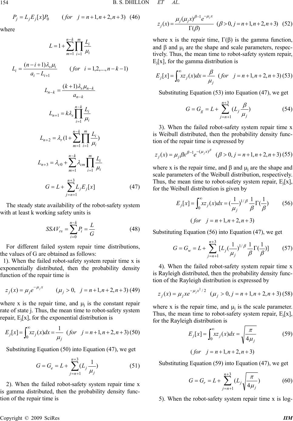

B. S. DHILLON ET AL. 154
)3,2,1(][0 nnnjforPxELPjjj (46)
where




kn
m
m
ii
i
L
L
11
1

)1,...,2,1(
)1(
1





knifor
La
in
L
ii
is
i

kn
kns
kn a
k
L





 )1(




kn
ii
i
sn
L
kL
1
1


)1(
11
2



kn
m
m
ii
i
rn
L
L







m
ii
i
kn
m
cmcn
L
L
1 1
03






3
1
][
n
nj
jj xELLG (47)
The steady state availability of the robot-safety system
with at least k working safety units is
G
L
PSSAV
kn
i
irs

0
(48)
For different failed system repair time distributions,
the values of G are obtained as follows:
1). When the failed robot-safety system repair time x is
exponentially distributed, then the probability density
function of the repair time is
)3,2,1,0()( nnnjexz j
x
jj
j


(49)
where x is the repair time, and j is the constant repair
rate of state j. Thus, the mean time to robot-safety system
repair, Ej[x], for the exponential distribution is
)3,2,1(
1
)(][
0
  nnnjfordxxxzxE
j
jj

(50)
Substituting Equation (50) into Equation (47), we get
)
1
(
3
1j
n
nj
je LLGG




 (51)
2). When the failed robot-safety system repair time x
is gamma distributed, then the probability density func-
tion of the repair time is
)3,2,1,0(
)(
)(
)(
1





nnnj
ex
xz
x
jj
j
j





(52)
where x is the repair time, () is the gamma function,
and  and j are the shape and scale parameters, respec-
tively. Thus, the mean time to robot-safety system repair,
Ej[x], for the gamma distribution is
)3,2,1()(][
0
  nnnjfordxxxzxE
j
jj


(53)
Substituting Equation (53) into Equation (47), we get
)(
3
1




n
nj j
jg LLGG


(54)
3). When the failed robot-safety system repair time x
is Weibull distributed, then the probability density func-
tion of the repair time is expressed by
)3,2,1,0()( )(
1  nnnjexxz x
jj
j




(55)
where x is the repair time, and  and j are the shape and
scale parameters of the Weibull distribution, respectively.
Thus, the mean time to robot-safety system repair, Ej[x],
for the Weibull distribution is given by
)
1
(
1
)
1
()(][ /1
0



j
jjdxxxzxE (56)
)3,2,1( 


nnnjfor
Substituting Equation (56) into Equation (47), we get
)]
1
(
1
)
1
([
3
1
/1




n
nj j
jw LLGG


(57)
4). When the failed robot-safety system repair time x
is Rayleigh distributed, then the probability density func-
tion of the Rayleigh distribution is expressed by
)3,2,1,0()( 2/
2 nnnjxexz j
x
jj
j


(58)
where x is the repair time, and j is the scale parameter.
Thus, the mean time to robot-safety system repair, Ej[x],
for the Rayleigh distribution is
j
jjdxxxzxE


4
)(][
0
 (59)
)3,2,1( 


nnnjfor
Substituting Equation (59) into Equation (47), we get
)
4
(
3
1




n
nj j
jr LLGG


(60)
5). When the robot-safety system repair time x is log-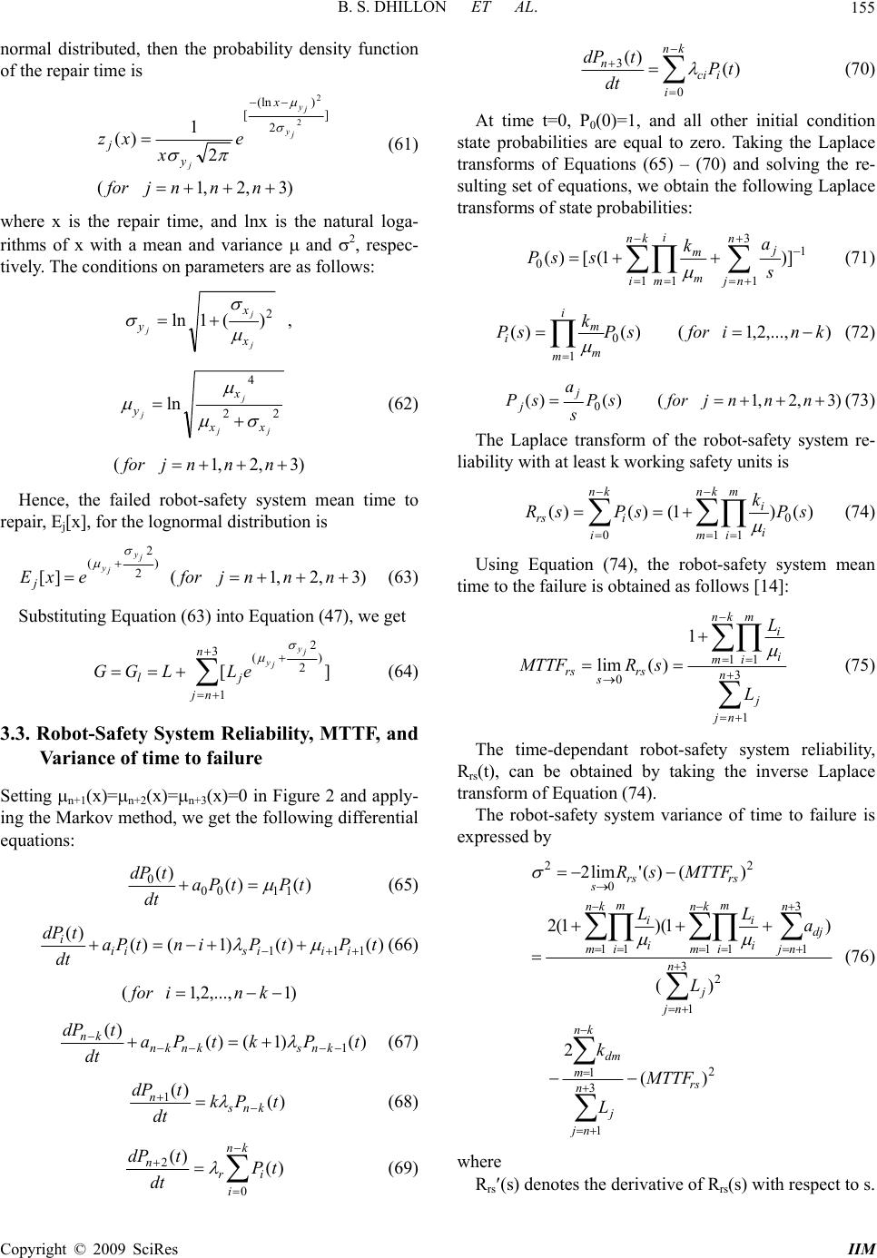

B. S. DHILLON ET AL. 155
normal distributed, then the probability density function
of the repair time is
)3,2,1(
2
1
)(
]
2
)(ln
[2
2



nnnjfor
e
x
xz j
y
j
y
j
x
y
j



(61)
where x is the repair time, and lnx is the natural loga-
rithms of x with a mean and variance  and 2, respec-
tively. The conditions on parameters are as follows:
,)(1ln 2
j
j
j
x
x
y


 
22
4
ln
jj
j
j
xx
x
y




 (62)
)3,2,1(  nnnjfor
Hence, the failed robot-safety system mean time to
repair, Ej[x], for the lognormal distribution is
)3,2,1(][ )
2
2
( nnnjforexE
j
y
j
y
j


(63)
Substituting Equation (63) into Equation (47), we get





3
1
)
2
2
(][
n
nj
jl
j
y
j
y
eLLGG


(64)
3.3. Robot-Safety System Reliability, MTTF, and
Variance of time to failure
Setting n+1(x)=n+2(x)=n+3(x)=0 in Figure 2 and apply-
ing the Markov method, we get the following differential
equations:
)()(
)(
1100
0tPtPa
dt
tdP
  (65)
)()()1()(
)(
111 tPtPintPa
dt
tdP
iiisii
i 
 (66)
)1,...,2,1(  knifor
)()1()(
)(
1tPktPa
dt
tdP
knsknkn
kn 
 (67)
)(
)(
1tPk
dt
tdP
kns
n 
 (68)




kn
i
ir
ntP
dt
tdP
0
2)(
)(
 (69)




kn
i
ici
ntP
dt
tdP
0
3)(
)(
 (70)
At time t=0, P0(0)=1, and all other initial condition
state probabilities are equal to zero. Taking the Laplace
transforms of Equations (65) – (70) and solving the re-
sulting set of equations, we obtain the following Laplace
transforms of state probabilities:
1
3
11 1
0)]1([)( 




n
nj
j
kn
i
i
mm
m
s
a
k
ssP

(71)
),...,2,1()()( 0
1
kniforsP
k
sP
i
mm
m
i 


(72)
)3,2,1()()( 0nnnjforsP
s
a
sP j
j(73)
The Laplace transform of the robot-safety system re-
liability with at least k working safety units is
)()1()()( 0
11 0
sP
k
sPsR
kn
m
m
ii
i
kn
i
irs 






(74)
Using Equation (74), the robot-safety system mean
time to the failure is obtained as follows [14]:








 3
1
11
0
1
)(lim n
nj
j
kn
m
m
ii
i
rs
s
rs
L
L
sRMTTF

(75)
The time-dependant robot-safety system reliability,
Rrs(t), can be obtained by taking the inverse Laplace
transform of Equation (74).
The robot-safety system variance of time to failure is
expressed by
2
3
1
1
2
3
1
11
3
111
2
0
2
)(
2
)(
)1)(1(2
)()('lim2
rs
n
nj
j
kn
m
dm
n
nj
j
kn
m
m
i
n
nj
dj
kn
m
m
ii
i
i
i
rsrs
s
MTTF
L
k
L
a
LL
MTTFsR























(76)
where
Rrs(s) denotes the derivative of Rrs(s) with respect to s.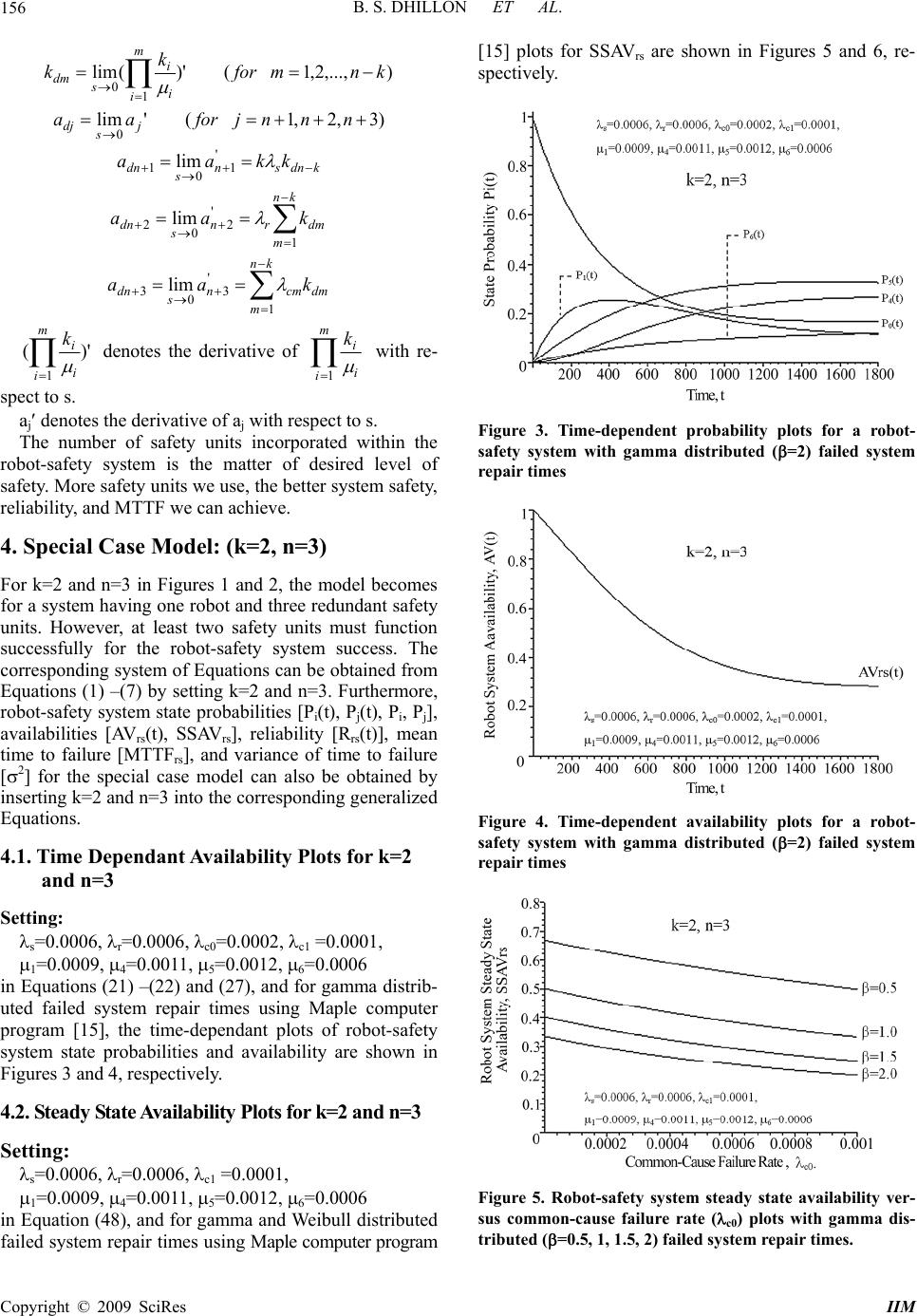

B. S. DHILLON ET AL. 156
),...,2,1()'(lim
1
0
knmfor
k
k
m
ii
i
s
dm  



)3,2,1('lim
0 nnnjforaa j s
dj
kdnsn
s
dn kkaa 



'
1
0
1lim






kn
m
dmrn
s
dn kaa
1
'
2
0
2lim







kn
m
dmcmn
s
dn kaa
1
'
3
0
3lim

)'(
1


m
ii
i
k

denotes the derivative of 

m
ii
i
k
1

with re-
spect to s.
aj denotes the derivative of aj with respect to s.
The number of safety units incorporated within the
robot-safety system is the matter of desired level of
safety. More safety units we use, the better system safety,
reliability, and MTTF we can achieve.
4. Special Case Model: (k=2, n=3)
For k=2 and n=3 in Figures 1 and 2, the model becomes
for a system having one robot and three redundant safety
units. However, at least two safety units must function
successfully for the robot-safety system success. The
corresponding system of Equations can be obtained from
Equations (1) –(7) by setting k=2 and n=3. Furthermore,
robot-safety system state probabilities [Pi(t), Pj(t), Pi, Pj],
availabilities [AVrs(t), SSAVrs], reliability [Rrs(t)], mean
time to failure [MTTFrs], and variance of time to failure
[2] for the special case model can also be obtained by
inserting k=2 and n=3 into the corresponding generalized
Equations.
4.1. Time Dependant Availability Plots for k=2
and n=3
Setting:
s=0.0006, r=0.0006, c0=0.0002, c1 =0.0001,
1=0.0009, 4=0.0011, 5=0.0012, 6=0.0006
in Equations (21) –(22) and (27), and for gamma distrib-
uted failed system repair times using Maple computer
program [15], the time-dependant plots of robot-safety
system state probabilities and availability are shown in
Figures 3 and 4, respectively.
4.2. Steady State Availability Plots for k=2 and n=3
Setting:
s=0.0006, r=0.0006, c1 =0.0001,
1=0.0009, 4=0.0011, 5=0.0012, 6=0.0006
in Equation (48), and for gamma and Weibull distributed
failed system repair times using Maple computer program
[15] plots for SSAVrs are shown in Figures 5 and 6, re-
spectively.
Figure 3. Time-dependent probability plots for a robot-
safety system with gamma distributed (=2) failed system
repair times
Figure 4. Time-dependent availability plots for a robot-
safety system with gamma distributed (=2) failed system
repair times
Figure 5. Robot-safety system steady state availability ver-
sus common-cause failure rate (c0) plots with gamma dis-
tributed (=0.5, 1, 1.5, 2) failed system repair times.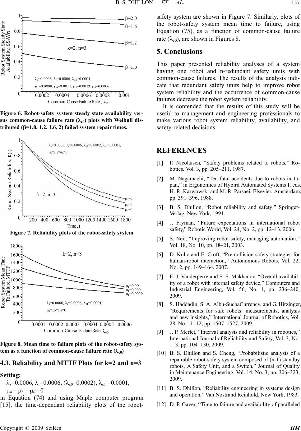

B. S. DHILLON ET AL. 157
Figure 6. Robot-safety system steady state availability ver-
sus common-cause failure rate (c0) plots with Weibull dis-
tributed (=1.0, 1.2, 1.6, 2) failed system repair times.
Figure 7. Reliability plots of the robot-safety system
Figure 8. Mean time to failure plots of the robot-safety sys-
tem as a function of common-cause failure rate (c0)
4.3. Reliability and MTTF Plots for k=2 and n=3
Setting:
s=0.0006, r=0.0006, (c0=0.0002), c1 =0.0001,
4 = 5 = 6= 0
in Equation (74) and using Maple computer program
[15], the time-dependant reliability plots of the robot-
safety system are shown in Figure 7. Similarly, plots of
the robot-safety system mean time to failure, using
Equation (75), as a function of common-cause failure
rate (c0), are shown in Figures 8.
5. Conclusions
This paper presented reliability analyses of a system
having one robot and n-redundant safety units with
common-cause failures. The results of the analysis indi-
cate that redundant safety units help to improve robot
system reliability and the occurrence of common-cause
failures decrease the robot system reliability.
It is contended that the results of this study will be
useful to management and engineering professionals to
make various robot system reliability, availability, and
safety-related decisions.
REFERENCES
[1] P. Nicolaisen, “Safety problems related to robots,” Ro-
botics, Vol. 3, pp. 205–211, 1987.
[2] M. Nagamachi, “Ten fatal accidents due to robots in Ja-
pan,” in Ergonomics of Hybird Automated Systems I, eds.
H. R. Karwowski and M. R. Parsaei, Elsevier, Amsterdam,
pp. 391–396, 1988.
[3] B. S. Dhillon, “Robot reliability and safety,” Springer-
Verlag, New York, 1991.
[4] J. Fryman, “Future expectations in international robot
safety,” Robotic World, Vol. 24, No. 2, pp. 12–13, 2006.
[5] S. Neil, “Improving robot safety, managing automation,”
Vol. 18, No. 10, pp. 18–21, 2003.
[6] D. Kulic and E. Croft, “Pre-collision safety strategies for
human-robot interaction,” Autonomous Robots, Vol. 22,
No. 2, pp. 149–164, 2007.
[7] E. J. Vanderperre and S. S. Makhanov, “Overall availabil-
ity of a robot with internal safety device,” Computers and
Industrial Engineering, Vol. 56, No. 1, pp. 236–240,
2009.
[8] S. Haddadin, S. A. Albu-SuchaCurrency, and G. Hirzinger,
“Requirements for safe robots: measurements, analysis
and new insights,” International Journal of Robotics, Vol.
28, No. 11–12, pp. 1507–1527, 2009.
[9] J. P. Merlet, “Interval analysis and reliability in robotics,”
International Journal of Reliability and Safety, Vol. 3, No.
1–3, pp. 104–130, 2009.
[10] B. S. Dhillon and S. Cheng, “Probabilistic analysis of a
repairable robot-safety system composed of (n-1) standby
robots, A Safety Unit, and a Switch,” Journal of Quality
in Maintenance Engineering, Vol. 14, No. 3, pp. 306–323,
2009.
[11] B. S. Dhillon, “Reliability engineering in systems design
and operation,” Van Nostrand Reinhold, New York, 1983.
[12] D. P. Gaver, “Time to failure and availability of paralleled

B. S. DHILLON ET AL. 158
systems with repair,” IEEE Transactions on Reliability,
Vol. 12, pp. 30–38, 1963.
[13] R. C. Grag, “Dependability of a complex system having
two types of components,” IEEE Transactions on Reli-
ability, Vol. 12, pp. 11–15, 1963.
[14] B. S. Dhillon, “Design reliability: fundamentals and ap-
plications,” CRC Press, Boca Raton, Florida, 1999.
[15] R. M. Corless, “Essential MAPLE: An introduction to
scientific programmers,” Springer–Verlag, New York,
1995.