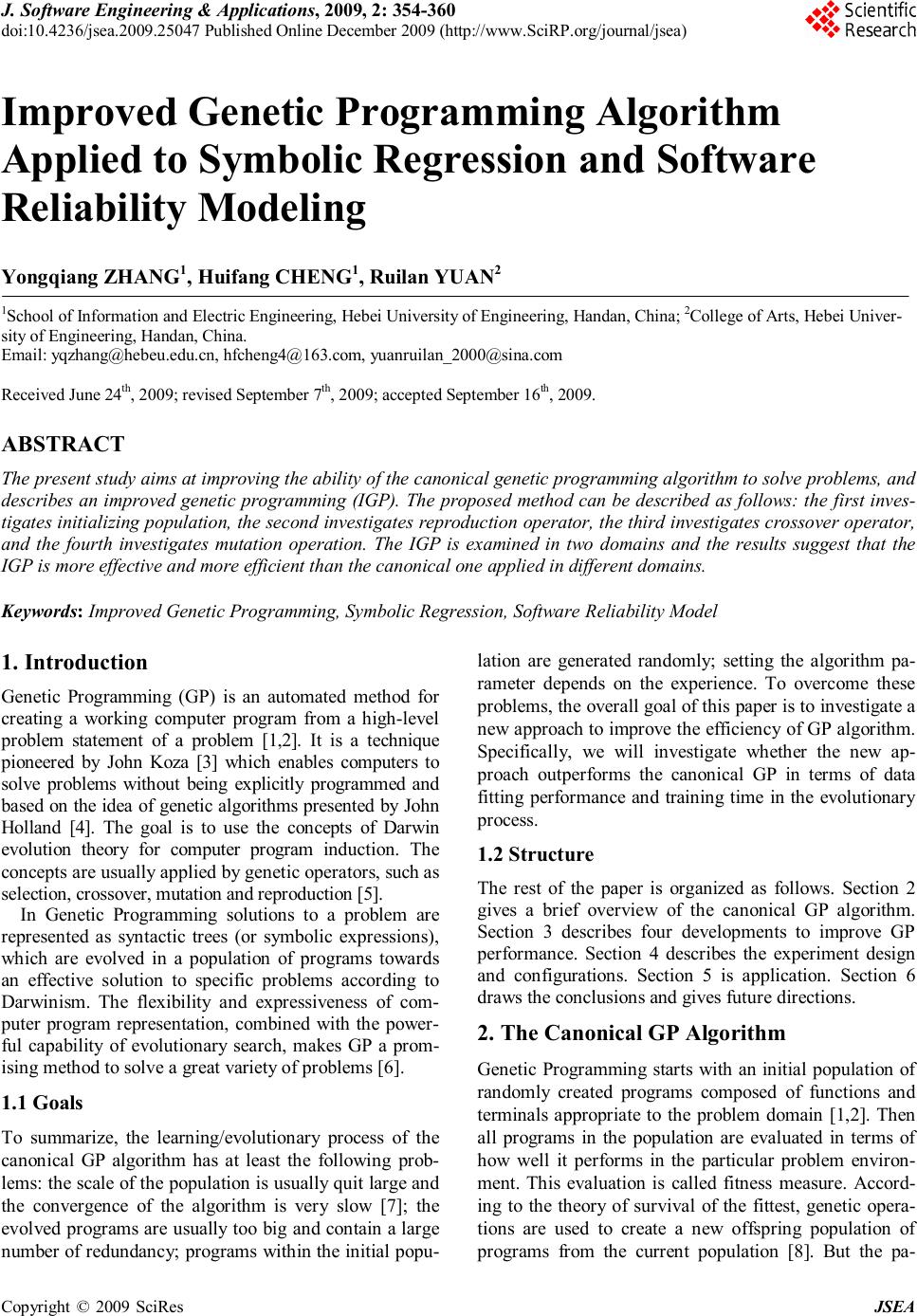J. Software Engineering & Applications, 2009, 2: 354-360
doi:10.4236/jsea.2009.25047 Published Online December 2009 (http://www.SciRP.org/journal/jsea)
Improved Genetic Programming Algorithm
Applied to Symbolic Regression and Software
Reliability Modeling
Yongqiang ZHANG1, Huifang CHENG1, Ruilan YUAN2
1School of Information and Electric Engineering, Hebei University of Engineering, Handan, China; 2College of Arts, Hebei Univer-
sity of Engineering, Handan, China.
Received June 24th, 2009; revised September 7th, 2009; accepted September 16th , 2009.
ABSTRACT
The present study aims at improving the ability of the canonical genetic programming algorithm to solve problems, and
describes an improved genetic programming (IGP). The proposed method can be described as follows: the first inves-
tigates initializing population, the second investigates reproduction operator, the third investigates crossover operator,
and the fourth investigates mutation operation. The IGP is examined in two domains and the results suggest that the
IGP is more effective and more efficient than the canonical one applied in different domains.
Keywords: Improved Genetic Programming, Symbolic Regression, Software Reliability Model
1. Introduction
Genetic Programming (GP) is an automated method for
creating a working computer program from a high-level
problem statement of a problem [1,2]. It is a technique
pioneered by John Koza [3] which enables computers to
solve problems without being explicitly programmed and
based on the idea of genetic algorithms presented by John
Holland [4]. The goal is to use the concepts of Darwin
evolution theory for computer program induction. The
concepts are usually applied by genetic operators, such as
selection, crossover, mutation and reproduction [5].
In Genetic Programming solutions to a problem are
represented as syntactic trees (or symbolic expressions),
which are evolved in a population of programs towards
an effective solution to specific problems according to
Darwinism. The flexibility and expressiveness of com-
puter program representation, combined with the power-
ful capability of evolutionary search, makes GP a prom-
ising method to solve a great variety of problems [6].
1.1 Goals
To summarize, the learning/evolutionary process of the
canonical GP algorithm has at least the following prob-
lems: the scale of the population is usually quit large and
the convergence of the algorithm is very slow [7]; the
evolved programs are usually too big and contain a large
number of redundancy; programs within the initial popu-
lation are generated randomly; setting the algorithm pa-
rameter depends on the experience. To overcome these
problems, the overall goal of this paper is to investigate a
new approach to improve the efficiency of GP algorithm.
Specifically, we will investigate whether the new ap-
proach outperforms the canonical GP in terms of data
fitting performance and training time in the evolutionary
process.
1.2 Structure
The rest of the paper is organized as follows. Section 2
gives a brief overview of the canonical GP algorithm.
Section 3 describes four developments to improve GP
performance. Section 4 describes the experiment design
and configurations. Section 5 is application. Section 6
draws the conclusions and gives future directions.
2. The Canonical GP Algorithm
Genetic Programming starts with an initial population of
randomly created programs composed of functions and
terminals appropriate to the problem domain [1,2]. Then
all programs in the population are evaluated in terms of
how well it performs in the particular problem environ-
ment. This evaluation is called fitness measure. Accord-
ing to the theory of survival of the fittest, genetic opera-
tions are used to create a new offspring population of
programs from the current population [8]. But the pa-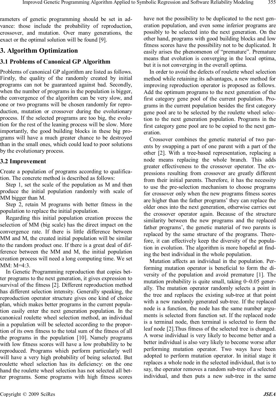

Improved Genetic Programming Algorithm Applied to Symbolic Regression and Software Reliability Modeling 355
rameters of genetic programming should be set in ad-
vance: those include the probability of reproduction,
crossover, and mutation. Over many generations, the
exact or the optimal solution will be found [9].
3. Algorithm Optimization
3.1 Problems of Canonical GP Algorithm
Problems of canonical GP algorithm are listed as follows.
Firstly, the quality of the randomly created by initial
programs can not be guaranteed against bad. Secondly,
when the number of programs in the population is bigger,
the convergence of the algorithm can be very slow, and
one or two programs will be chosen randomly for repro-
duction, mutation or crossover during the evolutionary
process. If the selected programs are too big, the evolu-
tion for the rest of the leaning process will be slow. More
importantly, the good building blocks in these big pro-
grams will have a much greater chance to be destroyed
than in the small ones, which could lead to poor solutions
by the evolutionary process.
3.2 Improvement
Create a population of programs according to qualifica-
tion. The concrete method is described as follows:
Step 1, set the scale of the population as M and then
produce the initial population randomly with scale of
MM bigger than M.
Step 2, retain M programs with better fitness in the
population to replace the initial population.
Regarding this initial population creation process the
selection of MM (big scale) has the direct impact on the
convergence rate. If there is little difference between
MM and M, the created initial population will be similar
to the random product one. If there is a great deal of dif-
ference between the MM and M, the initial population
creation process will need a long computing time. We set
MM: M=4:3.
In Genetic Programming reproduction that copies bet-
ter programs to the next generation, it gives expression to
survival of the fitness [2]. Different reproduction method
has different selection intensity. Generally speaking, the
reproduction operator structure gives one kind of choice
plan, which makes better programs in the current popula-
tion easily enter the next generation population. In the
canonical roulette wheel selection method, an individual
in a population will be selected according to the propor-
tion of its own fitness to the total sum of the fitness of all
the programs in the population [10]. Namely programs
with low fitness scores will have a low probability to be
reproduced. Programs which perform particularly well
will have a very high probability of being selected. But
roulette wheel selection has its deficiency: on the one
hand the roulette wheel selection has not selected all bet-
ter programs. Some programs with high fitness scores
have not the possibility to be duplicated to the next gen-
eration population, and even some inferior programs are
possibly to be selected into the next generation. On the
other hand, programs with good building blocks and low
fitness scores have the possibility not to be duplicated. It
easily arises the phenomenon of “premature”. Premature
means that evolution is converging in the local optima,
but it is not converging in the overall optima.
In order to avoid the defects of roulette wheel selection
method while retaining its advantages, a new method for
improving reproduction operator is proposed as follows.
Add the optimum programs to the next generation of the
first category gene pool of the current population. Pro-
grams in the current population besides the first category
gene pool are to be selected by the roulette wheel selec-
tion to the next generation population. Programs in the
first category gene pool are to be copied to the next gen-
eration.
Crossover combines the genetic material of two par-
ents by swapping a part of one parent with a part of the
other [2]. With a tree-based representation, replacing a
node means replacing the whole branch. This adds
greater effectiveness to the crossover operator. The ex-
pressions resulting from crossover are greatly different
from their initial parents. Therefore, it has the necessity
to use the pre-selection mechanism to choose programs
for crossover only when the new programs fitness scores
are higher than the father programs’ they can replace the
older ones into the next generation, otherwise carries out
the crossover operator again. Because of the structure
similarity between the new programs and the replaced
father programs’, the genetic material of two parents is
replaced by the same structure of the programs. There-
fore, it can effectively keep the diversity of the popula-
tion in evolution. The algorithm is more hopeful at find-
ing the best individual in the whole population.
Mutation affects an individual in the population. Per-
forming mutation operator is beneficial to form the di-
versity of the population and avoid premature [1]. The
mutation probability is quite small, taking 0~0.05 gener-
ally. The mutation operator randomly selects a point in
the tree and replaces the existing sub-tree at that point
with a new randomly generated sub-tree. If the replaced
node is a function, the node has the same number argu-
ments is selected from function set. If the replaced node
is a terminal node, then terminal is selected to form the
leaf node [2].Thus fitness of the selected tree is changed.
A worse individual is very likely to become better and a
better individual is also very likely to become worse after
performing mutation operator. Two ways have been
adopted to perform mutation operator. In initial stage it
replaces a whole node in the selected individual, that is to
say, the operator removes a random sub-tree of a selected
individual, and then puts a new sub-tree in the same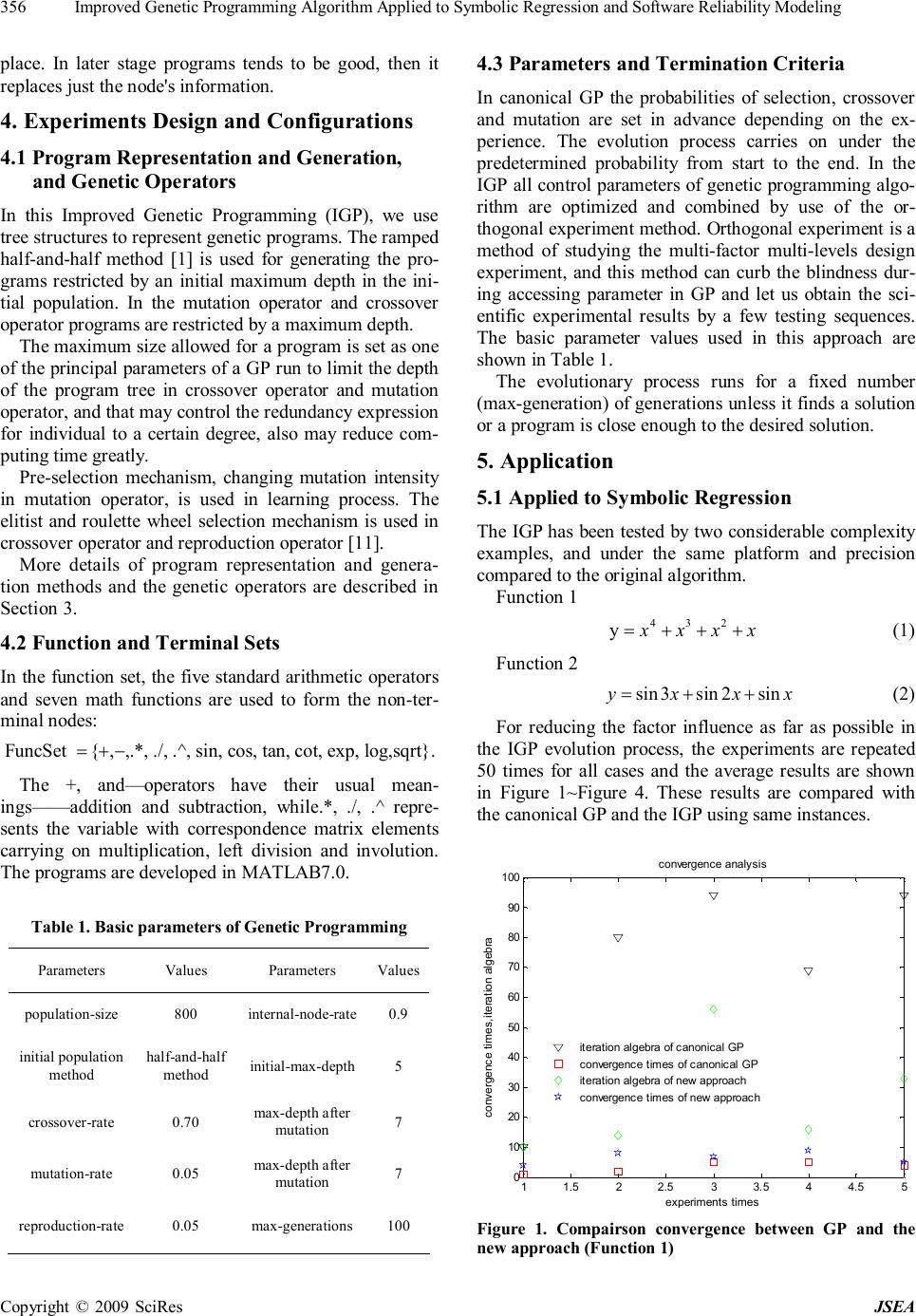

Improved Genetic Programming Algorithm Applied to Symbolic Regression and Software Reliability Modeling 356
place. In later stage programs tends to be good, then it
replaces just the node's information.
4. Experiments Design and Configurations
4.1 Program Representation and Generation,
and Genetic Operators
In this Improved Genetic Programming (IGP), we use
tree structures to represent genetic programs. The ramped
half-and-half method [1] is used for generating the pro-
grams restricted by an initial maximum depth in the ini-
tial population. In the mutation operator and crossover
operator programs are restricted by a maximum depth.
The maximum size allowed for a program is set as one
of the principal parameters of a GP run to limit the depth
of the program tree in crossover operator and mutation
operator, and that may control the redundancy expression
for individual to a certain degree, also may reduce com-
puting time greatly.
Pre-selection mechanism, changing mutation intensity
in mutation operator, is used in learning process. The
elitist and roulette wheel selection mechanism is used in
crossover operator and reproduction operator [11].
More details of program representation and genera-
tion methods and the genetic operators are described in
Section 3.
4.2 Function and Terminal Sets
In the function set, the five standard arithmetic operators
and seven math functions are used to form the non-ter-
minal nodes:
FuncSet {,,.*, ./, .^, sin, cos, tan, co
t, exp, log,sqrt}.
=+−
The +, and—operators have their usual mean-
ings——addition and subtraction, while.*, ./, .^ repre-
sents the variable with correspondence matrix elements
carrying on multiplication, left division and involution.
The programs are developed in MATLAB7.0.
Table 1. Basic parameters of Genetic Programming
Parameters Values Parameters Values
population-size 800 internal-node-rate 0.9
initial population
method half-and-half method initial-max-depth
5
crossover-rate 0.70 max-depth after
mutation 7
mutation-rate 0.05 max-depth after
mutation 7
reproduction-rate 0.05 max-generations 100
4.3 Parameters and Termination Criteria
In canonical GP the probabilities of selection, crossover
and mutation are set in advance depending on the ex-
perience. The evolution process carries on under the
predetermined probability from start to the end. In the
IGP all control parameters of genetic programming algo-
rithm are optimized and combined by use of the or-
thogonal experiment method. Orthogonal experiment is a
method of studying the multi-factor multi-levels design
experiment, and this method can curb the blindness dur-
ing accessing parameter in GP and let us obtain the sci-
entific experimental results by a few testing sequences.
The basic parameter values used in this approach are
shown in Table 1.
The evolutionary process runs for a fixed number
(max-generation) of generations unless it finds a solution
or a program is close enough to the desired solution.
5. Application
5.1 Applied to Symbolic Regression
The IGP has been tested by two considerable complexity
examples, and under the same platform and precision
compared to the original algorithm.
Function 1
432
y
xxxx
=+++
(1)
Function 2
sin3sin2sin
yxxx
=++ (2)
For reducing the factor influence as far as possible in
the IGP evolution process, the experiments are repeated
50 times for all cases and the average results are shown
in Figure 1~Figure 4. These results are compared with
the canonical GP and the IGP using same instances.
11.52 2.53 3.544.5 5
0
10
20
30
40
50
60
70
80
90
100
experiments times
convergence times,iteration algebra
convergence analysis
iteration algebra of canonical GP
convergence times of canonical GP
iteration algebra of new approach
convergence times of new approach
Figure 1. Compairson convergence between GP and the
new approach (Function 1)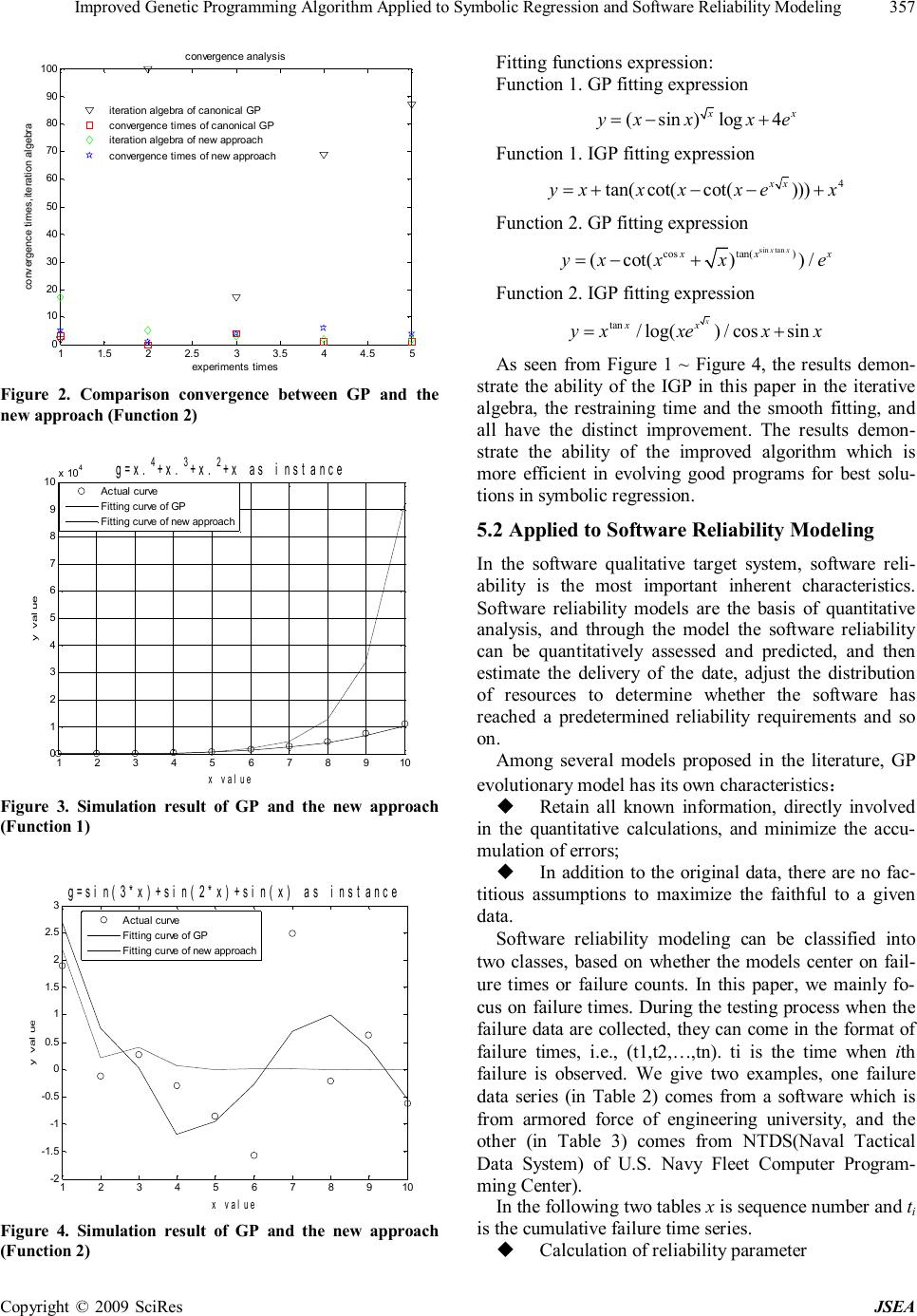

Improved Genetic Programming Algorithm Applied to Symbolic Regression and Software Reliability Modeling 357
11.5 2 2.533.5 4 4.5 5
0
10
20
30
40
50
60
70
80
90
100
experiments times
convergence times,iteration algebra
convergence analysis
iteration algebra of canonical GP
convergence times of canonical GP
iteration algebra of new approach
convergence times of new approach
Figure 2. Comparison convergence between GP and the
new approach (Function 2)
12345678910
0
1
2
3
4
5
6
7
8
9
10 x 104
x value
y value
g=x.
4
+x.
3
+x.
2
+x as instance
Actual curve
Fitting curve of GP
Fitting curve of new approach
Figure 3. Simulation result of GP and the new approach
(Function 1)
12345678910
-2
-1.5
-1
-0.5
0
0.5
1
1.5
2
2.5
3
x value
y value
g=sin(3*x)+sin(2*x)+sin(x) as instance
Actual curve
Fitting curve of GP
Fitting curve of new approach
Figure 4. Simulation result of GP and the new approach
(Function 2)
Fitting functions expression:
Function 1. GP fitting expression
(sin)log4
xx
yxxxe
=−+
Function 1. IGP fitting expression
4
tan(cot(cot()))
xx
yxxxxex
=+−−+
Function 2. GP fitting expression
sintan
costan()
(cot())/
xx
xxx
yxxxe
=−+
Function 2. IGP fitting expression
tan
/log()/cossin
x
xx
yxxexx
=+
As seen from Figure 1 ~ Figure 4, the results demon-
strate the ability of the IGP in this paper in the iterative
algebra, the restraining time and the smooth fitting, and
all have the distinct improvement. The results demon-
strate the ability of the improved algorithm which is
more efficient in evolving good programs for best solu-
tions in symbolic regression.
5.2 Applied to Software Reliability Modeling
In the software qualitative target system, software reli-
ability is the most important inherent characteristics.
Software reliability models are the basis of quantitative
analysis, and through the model the software reliability
can be quantitatively assessed and predicted, and then
estimate the delivery of the date, adjust the distribution
of resources to determine whether the software has
reached a predetermined reliability requirements and so
on.
Among several models proposed in the literature, GP
evolutionary model has its own characteristics：
u Retain all known information, directly involved
in the quantitative calculations, and minimize the accu-
mulation of errors;
u In addition to the original data, there are no fac-
titious assumptions to maximize the faithful to a given
data.
Software reliability modeling can be classified into
two classes, based on whether the models center on fail-
ure times or failure counts. In this paper, we mainly fo-
cus on failure times. During the testing process when the
failure data are collected, they can come in the format of
failure times, i.e., (t1,t2,…,tn). ti is the time when ith
failure is observed. We give two examples, one failure
data series (in Table 2) comes from a software which is
from armored force of engineering university, and the
other (in Table 3) comes from NTDS(Naval Tactical
Data System) of U.S. Navy Fleet Computer Program-
ming Center).
In the following two tables x is sequence number and ti
is the cumulative failure time series.
u Calculation of reliability parameter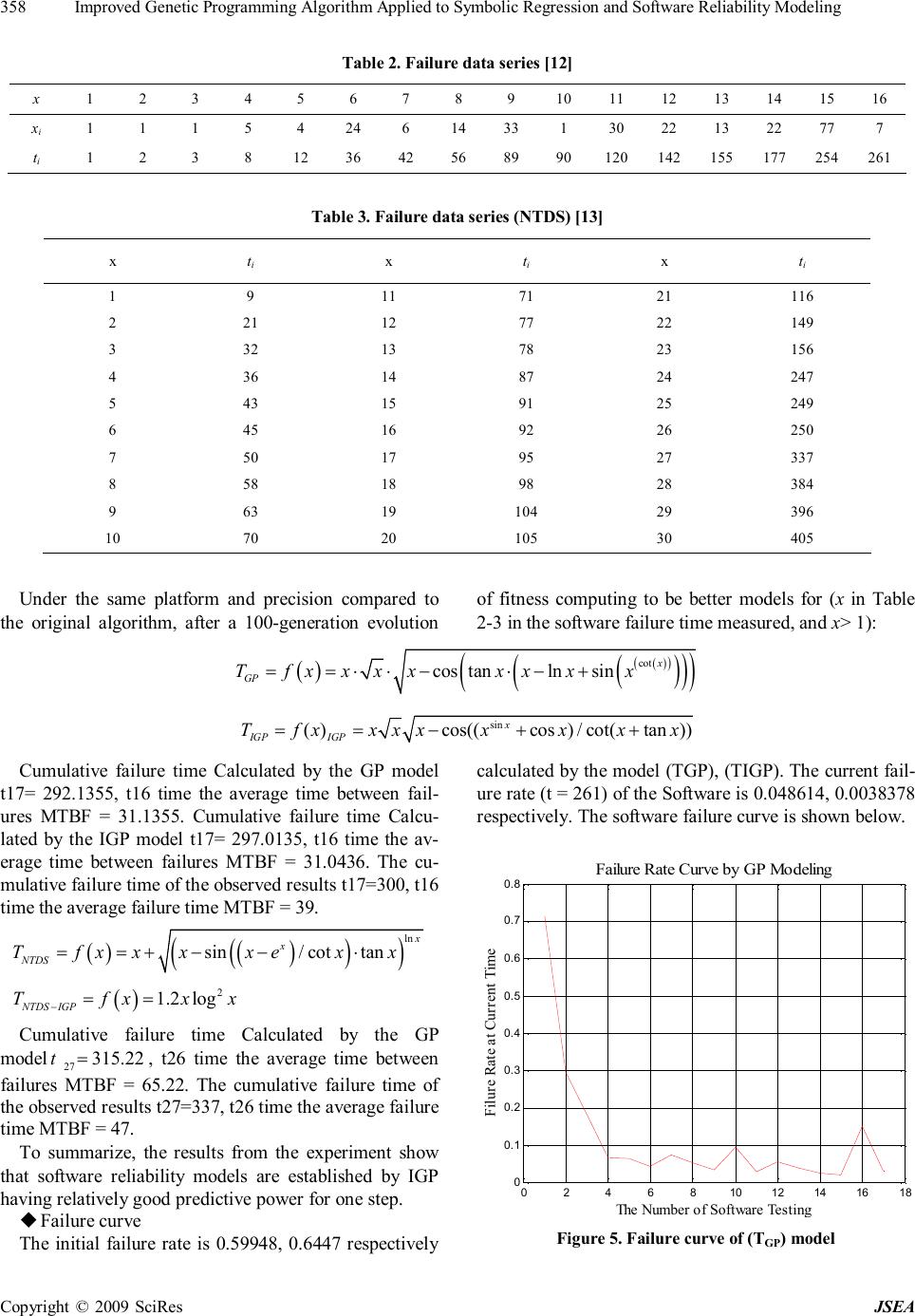

Improved Genetic Programming Algorithm Applied to Symbolic Regression and Software Reliability Modeling 358
Table 2. Failure data series [12]
x 1 2 3 4 5 6 7 8 9 10 11 12 13 14 15 16
xi 1 1 1 5 4 24 6 14 33 1 30 22 13 22 77 7
ti 1 2 3 8 12 36 42 56 89 90 120 142 155 177 254 261
Table 3. Failure data series (NTDS) [13]
x ti x ti x ti
1 9 11 71 21 116
2 21 12 77 22 149
3 32 13 78 23 156
4 36 14 87 24 247
5 43 15 91 25 249
6 45 16 92 26 250
7 50 17 95 27 337
8 58 18 98 28 384
9 63 19 104 29 396
10 70 20 105 30 405
Under the same platform and precision compared to
the original algorithm, after a 100-generation evolution of fitness computing to be better models for (x in Table 2-3 in the software failure time measured, and x> 1):
()
() ( )
(
)
(
)
(
)
cot
costanlnsin x
GP
Tfxxxxxxxx==⋅⋅−⋅−+
sin
()cos((cos)/cot(tan))
x
IGPIGP
Tfxxxxxxxx
==−++
Cumulative failure time Calculated by the GP model
t17= 292.1355, t16 time the average time between fail-
ures MTBF = 31.1355. Cumulative failure time Calcu-
lated by the IGP model t17= 297.0135, t16 time the av-
erage time between failures MTBF = 31.0436. The cu-
mulative failure time of the observed results t17=300, t16
time the average failure time MTBF = 39.
()
( )
( )
( )
ln
sin/cottan
x
x
NTDS
Tfxxxxexx==+−−⋅
(
)
2
1.2log
NTDSIGP
Tfxxx
−==
Cumulative failure time Calculated by the GP
model 27
315.22
t=, t26 time the average time between
failures MTBF = 65.22. The cumulative failure time of
the observed results t27=337, t26 time the average failure
time MTBF = 47.
To summarize, the results from the experiment show
that software reliability models are established by IGP
having relatively good predictive power for one step.
u Failure curve
The initial failure rate is 0.59948, 0.6447 respectively
calculated by the model (TGP), (TIGP). The current fail-
ure rate (t = 261) of the Software is 0.048614, 0.0038378
respectively. The software failure curve is shown below.
0246810 12 14 1618
0
0.1
0.2
0.3
0.4
0.5
0.6
0.7
0.8
The Number of Software Testing
Filure Rate at Current Time
Failure Rate Curve by GP Modeling
Figure 5. Failure curve of (TGP) model

Improved Genetic Programming Algorithm Applied to Symbolic Regression and Software Reliability Modeling 359
0246810 12 14 16
18
0
0.1
0.2
0.3
0.4
0.5
0.6
0.7
0.8
0.9
1
The Number of Software Testing
Filure Rate at Current Time
Failure Rate Curve by IGP Modeling
Figure 6. Failure curve of (TIGP) model
05 10 15 2025
30
0
0.1
0.2
0.3
0.4
0.5
0.6
0.7
0.8
The Number of Software Testing
Filure Rate at Current Time
Failure Rate Curve by GP Modeling
Figure 7. Failure curve of (TNTDS) model
0510 1520 2530
0
0.5
1
1.5
The Number of Software Testing
Filure Rate at Current Time
Failure Rate Curve by IGP Modeling
Figure 8. Failure curve of (TNTDS-IGP) model
0246810 12 14 1618
0
50
100
150
200
250
300
Software Testing Serial Number
Cumulative Failure Time
Data from Armored Force of Engineering University
evolved by GP
evolved by IGP
real failure data series
Figure 9. Simulation result of GP and IGP model
0510 15 20 25
30
0
50
100
150
200
250
300
350
400
450
Software Testing Serial Number
Cumulative Failure Time
Data from NTDS
evolved by GP
evolved by IGP
real failure data series
Figure 10. Simulation result of GP and IGP model
The initial failure rate is 0.5、0.24869 respectively
calculated by the model (TNTDS), (TNTDS-IGP). The
current failure rate (t = 405) of the Software is
0.0026775、0.0022268 respectively. The software failure
curve is shown above.
u Model simulation
Simulation studies are presented to validate the models.
The results show that the models set up by IGP are better
than the models set up by the canonical algorithms.
According to the theoretical and experimental analysis,
our IGP algorithm not only provides the same excellent
performance as the canonical GP, but also can save con-
siderable convergence time against canonical GP.
6. Conclusions
GP is a powerful paradigm that can be used to solve dif-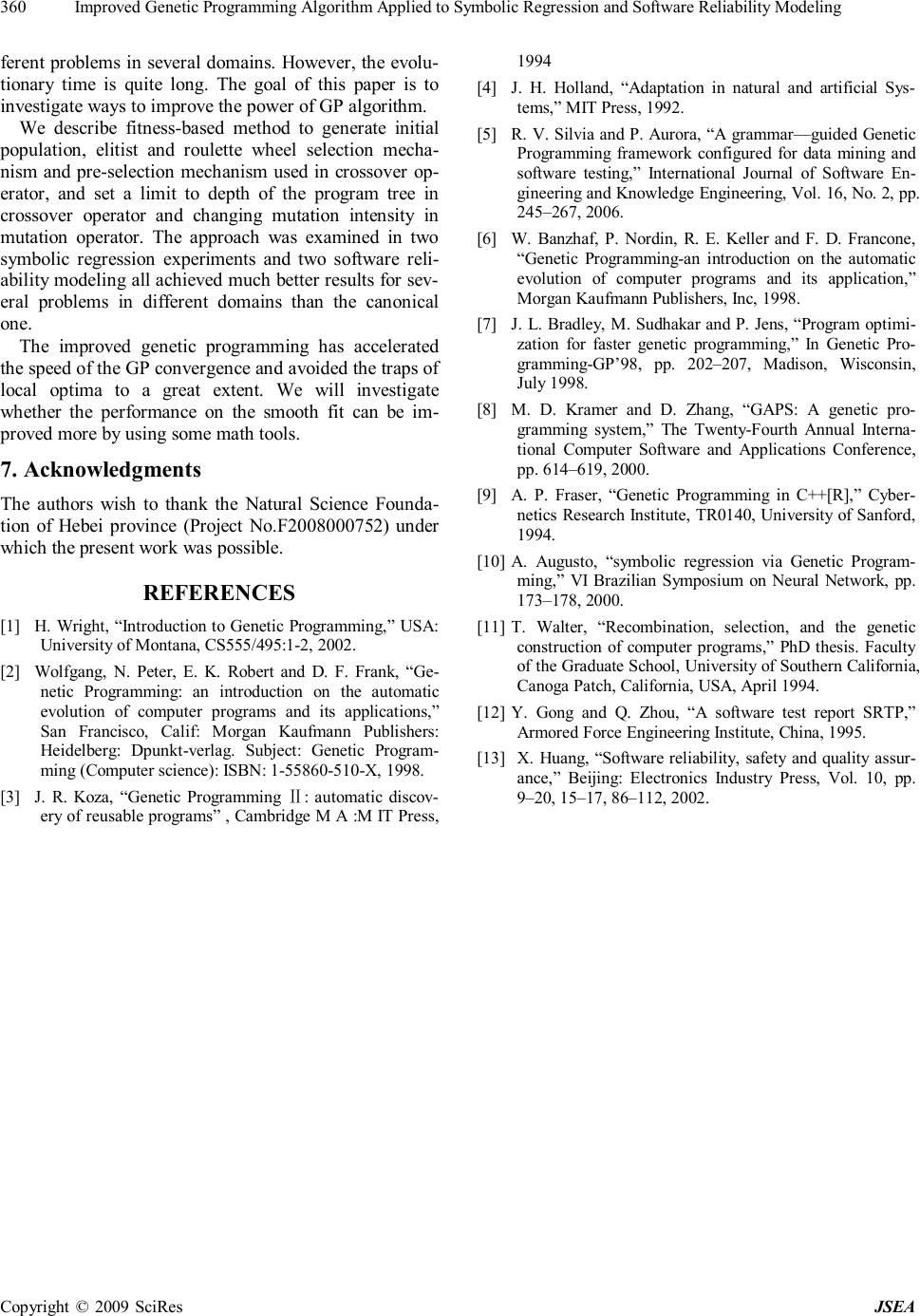

Improved Genetic Programming Algorithm Applied to Symbolic Regression and Software Reliability Modeling 360
ferent problems in several domains. However, the evolu-
tionary time is quite long. The goal of this paper is to
investigate ways to improve the power of GP algorithm.
We describe fitness-based method to generate initial
population, elitist and roulette wheel selection mecha-
nism and pre-selection mechanism used in crossover op-
erator, and set a limit to depth of the program tree in
crossover operator and changing mutation intensity in
mutation operator. The approach was examined in two
symbolic regression experiments and two software reli-
ability modeling all achieved much better results for sev-
eral problems in different domains than the canonical
one.
The improved genetic programming has accelerated
the speed of the GP convergence and avoided the traps of
local optima to a great extent. We will investigate
whether the performance on the smooth fit can be im-
proved more by using some math tools.
7. Acknowledgments
The authors wish to thank the Natural Science Founda-
tion of Hebei province (Project No.F2008000752) under
which the present work was possible.
REFERENCES
[1] H. Wright, “Introduction to Genetic Programming, ” USA:
University of Montana, CS555/495:1-2, 2002.
[2] Wolfgang, N. Peter, E. K. Robert and D. F. Frank, “Ge-
netic Programming: an introduction on the automatic
evolution of computer programs and its applications, ”
San Francisco, Calif: Morgan Kaufmann Publishers:
Heidelberg: Dpunkt-verlag. Subject: Genetic Program-
ming (Computer science): ISBN: 1-55860-510-X, 1998.
[3] J. R. Koza, “Genetic Programming : automatic discoⅡv-
ery of reusable programs” , Cambridge M A :M IT Press,
1994
[4] J. H. Holland, “Adaptation in natural and artificial Sys-
tems, ” MIT Press, 1992.
[5] R. V. Silvia and P. Aurora, “A grammar—guided Genetic
Programming framework configured for data mining and
software testing, ” International Journal of Software En-
gineering and Knowledge Engineering, Vol. 16, No. 2, pp.
245–267, 2006.
[6] W. Banzhaf, P. Nordin, R. E. Keller and F. D. Francone,
“Genetic Programming-an introduction on the automatic
evolution of computer programs and its application,”
Morgan Kaufmann Publishers, Inc, 1998.
[7] J. L. Bradley, M. Sudhakar and P. Jens, “Program optimi-
zation for faster genetic programming, ” In Genetic Pro-
gramming-GP’98, pp. 202–207, Madison, Wisconsin,
July 1998.
[8] M. D. Kramer and D. Zhang, “GAPS: A genetic pro-
gramming system,” The Twenty-Fourth Annual Interna-
tional Computer Software and Applications Conference,
pp. 614–619, 2000.
[9] A. P. Fraser, “Genetic Programming in C++[R],” Cyber-
netics Research Institute, TR0140, University of Sanford,
1994.
[10] A. Augusto, “symbolic regression via Genetic Program-
ming, ” VI Brazilian Symposium on Neural Network, pp.
173–178, 2000.
[11] T. Walter, “Recombination, selection, and the genetic
construction of computer programs,” PhD thesis. Faculty
of the Graduate School, University of Southern California,
Canoga Patch, California, USA, April 1994.
[12] Y. Gong and Q. Zhou, “A software test report SRTP,”
Armored Force Engineering Institute, China, 1995.
[13] X. Huang, “Software reliability, safety and quality assur-
ance,” Beijing: Electronics Industry Press, Vol. 10, pp.
9–20, 15–17, 86–112, 2002.