Paper Menu >>
Journal Menu >>
 J. Software Engineering & Applications, 2009, 2: 344-349 doi:10.4236/jsea.2009.25045 Published Online December 2009 (http://www.SciRP.org/journal/jsea) Copyright © 2009 SciRes JSEA Research on OD Matrix Calculation Based on Quantum Behaved Particle Swarm Optimization Algorithm Lianyu WEI, Jianfu DU Institute of Civil Engineering, Hebei University of Technology, Tianjin, China. Email: {wly57, batdujianfu}@126.com Received June 20th, 2009; revised August 25th, 2009; accepted September 2nd, 2009. ABSTRACT Traffic information is so far less than the number of OD variables, that it is difficult to obtain the satisfactory solution. In this paper, a method based on Quantum behaved Particle Swarm Optimization (QPSO) algorithm is developed to obtain the global optimal solution. It designs the method based on QPSO algorithm to solve the OD matrix prediction model, lists the detailed steps and points out how to choose the PSO operator. Moreover, it uses MATLAB program- ming language to carry out the simulation test. The simulation results show that the method has higher efficiency and accuracy. Keywords: OD Matrix Prediction Model, QPSO, Simulation Analysis, Optimal Design 1. Introduction The traffic between import and export at the intersection is an important data for urban traffic management and control, and also impacts on the control of traffic lights at the intersection directly. Therefore, how to obtain accu- rate intersection OD and avoid the time-delay of control and decision-making system are very important issues. As the OD matrix calculation based on traffic has advantages, such as convenience, rapidness, low-cost, effectiveness, it has been more and more used in transport planning re- cently. However, when the number of surveyed sections is less than the number of OD variables, the solution of OD matrix calculation will be non-unique and cannot guarantee the accuracy [1]. Moreover, the objective func- tion and fitness function of OD matrix calculation are mostly nonlinear equations. In light of the above issues, taking the reality situation that observation error and ran- dom error exist into account, the relationship between OD traffic and road traffic is not absolute linear. Although through rigorous mathematical methods, it cannot get an exact solution to the problem. In pursuit of finding solution to these problems many researchers have been drawing ideas from the field of biology. A host of such biologically inspired evolutionary techniques have been developed namely Genetic Algo- rithm (GA) ([Baykasoğlu et al., 2008], [Costa et al., 2004], [Grosset et al., 2001], [Gürdal Soremekun et al., 2001], [Le Riche and Haftka, 1993], [Park et al., 2001], [Rajen- dran and Vijayarangan, 2001] and [Walker and Smith, 2003]), Artificial Neural Networks (ANN) (Garg, Roy Mahapatra, Suresh, Gopalakrishna & Omkar, 2007), Arti- ficial Immune System (AIS) (Omkar, Khandelwal, San- thosh Yathindra, Narayana Naik & Gopalakrishna, 2008) and Particle Swarm Optimization (PSO) (Omkar, Mud- igere, Narayana Naik & Gopalakrishna, 2008; Parsopou- los, Tasoulis & Vrahatis, 2004) which are widely used for solving such optimization problems. All of these algo- rithms with their stochastic means are well equipped to handle such problems [2]. Particle Swarm Optimization was introduced by Eber- hart and Kennedy [3], inspired by the social behavior of animals such as bird flocking, fish schooling, and the swarm theory. Compared with GA and other similar evo- lutionary techniques, PSO has some attractive characteris- tics and in many cases proved to be more effective (Has- san, Cohanim, Weck & Venter, 2005). Both GA and PSO have been used extensively for a variety of optimization problems and in most of these cases PSO has been proven to have superior computational efficiency ([Hassan et al., 2005] and [Sun, 2008]; Zhang et al., 2003 L. B. Zhang, C. G. Zhou, X. H. Liu, Z. Q. Ma, M. Ma & Y. C. Liang (2003) solved multi-objective optimization problems us- ing particle swarm optimization in Proceedings of the IEEE congress on evolutionary computation (CEC). Since  Research on OD Matrix Calculation Based on Quantum Behaved Particle Swarm Optimization Algorithm Copyright © 2009 SciRes JSEA 345 1995, many attempts have been made to improve the per- formance of the PSO (Clerc, 2004; Zheng, Ma, & Zhang, 2003). (Sun et al., 2004) and (Sun and Xu et al., 2004) introduced quantum theory into PSO and proposed a Quantum-behaved PSO (QPSO) algorithm, which are guaranteed theoretically to find good optimal solutions in search of space. The experiment results on some widely used benchmark functions show that the QPSO works better than standard PSO ([Sun et al., 2004] and [Sun and Xu et al., 2004]) and is a promising algorithm. Hence in the current work we propose to employ a multi objective optimization method based on QPSO and compare it to its predecessor PSO, which has been already implemented by Omkar and Mudigere et al. (2008) [2]. This paper firstly establishes maximum entropy OD matrix calculation model. It makes full use of the quan- tum behaved particle swarm optimization algorithm (QPSO algorithm) to solve the global optimization of the objective function, lists the detailed steps of calculation and shows how to choose the particle swarm operator, and then calculates the OD matrix of road intersection. Finally, compared to the results of conventional PSO al- gorithm, it verifies the superiority of QPSO algorithm. Therefore, this paper provides a more reliable method to solve the OD matrix of road intersection. 2. Origin—Destination Matrix Prediction Model 2.1 Maximum Entropy Model The maximum entropy approach is motivated by ‘infor- mation theory’ and the work of Shannon, 1948. C. E. Shannon, A mathematical theory of communication. Bell Syst. Tech. J. (1948), pp. 379–423. Shannon (1948) who defined a function to measure the uncertainty, or entropy, of a collection of events, and Jaynes who proposed maximizing that function subject to appropriate consis- tency relations, such as moment conditions. The maxi- mum entropy (ME) principle and its sister formulation, minimum cross-entropy (CE), are now used in a wide variety of fields to estimate and make inferences when information is incomplete, highly scattered, and/or incon- sistent (Kapur and Kesavan, 1992). In economics, the ME principle has been successfully applied to a range of econometric problems, including nonlinear problems, where limited data and/or computational complexity hin- der traditional estimation approaches. Theil (1967) pro- vides an early investigation of information theory in eco- nomics. Mittelhammer et al. (2000) provide a recent text book treatment which is focused more tightly on the ME principle and its relationships with more traditional esti- mation criteria such as maximum likelihood [4]. In general, information in an estimation problem using the entropy principle comes in two forms: 1) information (theoretical or empirical) about the system that imposes constraints on the values that the various parameters can take; and 2) prior knowledge of likely parameter values. In the first case, the information is applied by specifying constraint equations in the estimation procedure. In the second, the information is applied by specifying a discrete prior distribution and estimating by minimizing the en- tropy distance between the estimated and prior distribu- tions — the minimum Cross-Entropy (CE) approach. The prior distribution does not have to be symmetric and weights on each point in the prior distribution can vary. If the weights in the prior distribution are equal (e.g. the prior distribution is uniform), then the CE and ME ap- proaches are equivalent. The model is as follows: ( ) maxlnln 11 nn ETTT ijij ij =−− ∑∑ == (1) 11 ..1,, nn k kijij ij stVTPkm == == ∑∑ L (2) 0, ij Tij ≥∀ (3) 11 nn ij ij TT == = ∑∑ (4) Where n is the number of OD pairs; ij T is the estimated OD matrix; k V is the detected traffic on section k; k ij p is the distribution ratio of ij T on section k, which is obtained by the traffic distribution. 2.2 Hopfield Neural Network Model The Hopfield Neural Network model [4] is ( ) 1 , ,1,2,,. N ii iijj j ii duU CITV dtR VguiN = =−++ == ∑ K (5) Here in Equation (5), ij T is the connection weight value between node I and node J , and ijji TT = ; ( ) g ⋅ . is a function with ( ) 0 g′ ⋅> ; i U is the input of node I; i V is the output of node I ; i I is the constant value of node I ; C is a positive constant; and R is a positive constant. Equation (5) can be abbreviated to be ( ) 1 , ,1,2,,. N iiijj j ii du ITV dt VguiN = =+ == ∑ K (6) It can be proved that when the energy function of sys- tem (6) is 111 1 2 NNN ijijii iji ETVVVI === =−− ∑∑∑ We can have 0 dE dt ≤ , and only when 0 i dVdt = ,  Research on OD Matrix Calculation Based on Quantum Behaved Particle Swarm Optimization Algorithm Copyright © 2009 SciRes JSEA 346 0 dEdt = , ( ) 1,2,, iN = K . The stable state of system (6) is the local minimum of the above energy function. The computation processor of system (6) is a process to find the local minimum in fact, the goal function is the above energy function of system (6). Maximum entropy model is recognized by majority of scholars among many OD matrix calculation models, be- cause this model’s structure is simple and principle is clear. It also suits the situation without a priori OD matrix and which is a congested network [5]. 2.3 Model Simplification In light of above optimization problems, it is difficult to solve the objective function directly. So Lagrange multi- plier method is used to obtain the Lagrange function L: 11111 (lnln)() nnmnn k ijijkkijij ijkij LTTTVTP λ ===== =−−+− ∑∑∑∑∑ (7) The following Equation is the result of the first-Order derivative of ij T 1 ln0 m ij k kij k ij T LP TT λ = ∂ =−−= ∂∑ (8) So, 1 exp() m k ijkij k TTP λ = =− ∑ (9) T is given as 0 exp() T λ =−and take it into the Equa- tions (7) and (9) respectively. The results are as follows: 111 0 111 exp()1 exp() nnm k kij ijk nnm kk ijkijk ijk P PPV λ λλ === === −= −−= ∑∑∑ ∑∑∑ 1,, km = L (10) Above equations are a set of nonlinear equations. The number of variables is (m+1) which is equivalent to the number of equations. Lagrange multipliers: 01 , m λλλ LL can be solved. And then the OD matrix can be obtained according to Equation (9). 3. Design of the Quantum Behaved Particle Swarm Optimization Algorithm 3.1 Particle Swarm Optimization Algorithm Particle Swarm Optimization algorithm is a global opti- mization algorithm that can reproduce swarm intelligence. It is inspired from the foraging behavior of animal groups. When groups search for the optimal target, each individ- ual searches for its own goal. At the same time, individual refers to other individuals who have achieved optimal location and then adjusts the next search. The algorithm uses the speed-location search model. The current loca- tion of No.i particle is defined as i X =12 (,,...) iiid xxx , experienced position is defined as i P=12 (,,...) iiid ppp . Fitness function determines the level of merits of the lo- cation, while fitness function is determined by the opti- mization goal. Where, the individual particle best position is abbreviated as pbest , and the best location that all par- ticles have experienced is regarded as global best location ( gbest ). The speed of No. i particle is defined as 12 (,,...) iiiid Vvvv =that is the distance each iterative parti- cle moves. The Equations of conventional PSO algorithm are described as follows: 11122 ()() iiii vvrpbestxrgbestx φφ + =+⋅⋅−+⋅⋅− (11) 11 iii xxv ++ =+ (12) 3.2 Quantum Behaved Particle Swarm Optimization Algorithm Particle Swarm Optimization algorithm is based on the theory of swarm intelligence optimization algorithm. As in the classical system, particles achieve convergence in the form of orbit. Moreover, the speed of particles is lim- ited, and the space of particles is also a limited region that can not cover the entire feasible space. Therefore, with the quantum mechanics’ point of view that particles have quantum behavior, QPSO (Quantum Particle Swarm Op- timization) algorithm is proposed [3,7–8]. Particle swarm achieves iterative update through the following four Equations: 1 12 111 / /,/,,/ M i i MMM iiid iii mbsetpbestM pbestMpbestMpbestM = === = = ∑ ∑∑∑ L (13) ( ) maxminmax max T T ββ ββ −⋅ =− (14) 1212 ()/() prpbestrgbestrr =⋅+⋅+ (15) ()ln(1/)0.5 (1) ()ln(1/)0.5 pmbestxtuifu xt pmbestxtuifu β β +×−×< += −×−×≥ (16) In order to avoid algorithm premature, Mean Best Posi- tion (mbest) is regarded as the barycenter of all particles. Where, i pbest is the best position of the particle. β is the contraction and expansion coefficient that impacts the convergence speed and performance of algorithm. In this paper, deal with β by adaptive changes in accordance with Equation (14). T is the number of current iteration. Tmax is the maximum number of iterations. 12 , rr ∈  Research on OD Matrix Calculation Based on Quantum Behaved Particle Swarm Optimization Algorithm Copyright © 2009 SciRes JSEA 347 (0,1) rand , gbest is the global optimal solution, u ∈ (0,1) rand . 3.3 Optimal Design of Origin—Destination Matrix Calculation Model Algorithm Algorithm design, including as follows: 1) the determination of objective function In order to obtain better accuracy, this problem will be translated into the following optimization problem. The optimizing goal is that minimizes the mean square devia- tion of the calculated value of the left from the true value of the right in Equation (13). That is: 0 ()() min() 1 m kkkk k vVvV Jm λ= −⋅− =+ ∑ (17) Where, 0111 exp() nnm kk ijkij ijk vPP λ === =− ∑∑∑ 0 1 V = 0 111 exp(),1,... nnm kk kijkij ijk vPPkm λλ === =−−= ∑∑∑ Lagrange multipliers 01 , m λλλ LL are unknown. So- lution space is the range of Lagrange multipliers. Because the Lagrange multipliers are not given in this model ex- plicitly, it is necessary to estimate conservatively accord- ing to the specific issues and enlarge the range appropri- ately. 2) detailed implementation steps are: Step1: Initialize particle swarm. Step2: Calculate the value of particle objective func- tion. Step3: Update pbest and gbest according to parti- cles’ fitness. Step4: Calculate mbest according to Equation (13). Step5: Calculate random point p of each particle ac- cording to Equation (15). Step6: Calculate new location of each particle accord- ing to Equation (16). Step7: Double counting, until meet the number of itera- tions. 3.4 Simulation of a Typical Function Optimization Now, QPSO algorithm is illustrated that can be applied to the circuit performance equation to solve the global minimum feasibility and effectively, by solving the Schaffer’s f6 function. The value of the global minimum is 0. The Schaffer’s f6 function is: 222 2222 sin0.5 (,)0.5 (10.001()) xy fxy xy +− =+ +×+ (18) (10,10) x∈− ; (10,10) y∈− Use QPSO algorithm and PSO algorithm to solve the above equation respectively. The selected parameters are as follows: Particle number is 10; the maximum number of iterations is 1000; the ac- curacy is set to 1e-25. Figure 1 and Figure 2 show the obtained convergence curves. As can be seen from Figure 1, when the iteration num- ber reached 210, the curve tends to converge. Whereas, when the iteration number reached 310, the curve of Fig- ure 2 tends to converge; the solution of QPSO algorithm from Figure 1 is 0, while, the solution of PSO algorithm from Figure 2 is 0.000114686. Therefore, this example shows that the convergence speed and accuracy of QPSO algorithm are far better than the PSO algorithm for opti- mization problems. 4. Simulation Examples 4.1 Simulation Results This paper uses MATLAB programming language to carry out the simulation test. The intersection is shown in Figure 3. The traffic of every import is regarded as x1, x2, x3, x4 respectively. The traffic of every export is regarded as y1, y2, y3, y4 respectively. The traffic at intersection can be obtained by the detector. Count the total number of observed vehicles from 8:00 a.m. to 8:00 p.m. Figure 1. Convergence curve of QPSO algorithm Figure 2. Convergence curve of PSO algorithm 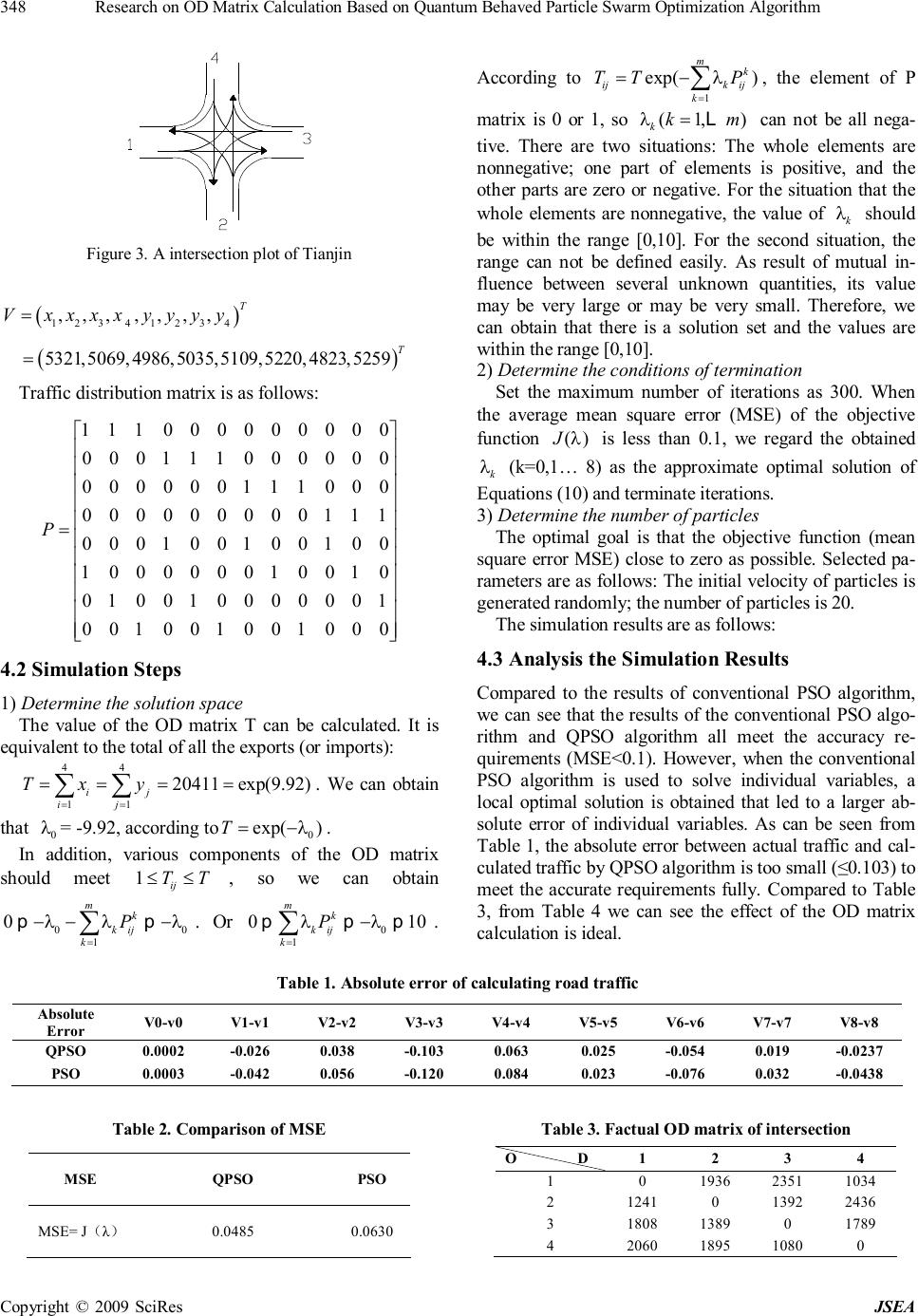 Research on OD Matrix Calculation Based on Quantum Behaved Particle Swarm Optimization Algorithm Copyright © 2009 SciRes JSEA 348 Figure 3. A intersection plot of Tianjin ( ) 12341234 ,,,,,,, T Vxxxxyyyy = ( ) 5321,5069,4986,5035,5109,5220,4823,5259 T = Traffic distribution matrix is as follows: 111000000000 000111000000 000000111000 000000000111 000100100100 100000010010 010010000001 001001001000 P = 4.2 Simulation Steps 1) Determine the solution space The value of the OD matrix T can be calculated. It is equivalent to the total of all the exports (or imports): 44 11 20411exp(9.92) ij ij Txy == ==== ∑∑ . We can obtain that 0 λ = -9.92, according to 0 exp() T λ =−. In addition, various components of the OD matrix should meet 1ij TT ≤≤ , so we can obtain 00 1 0mk kij k P λλλ = −−− ∑ pp. Or 0 1 010 mk kij k Pλλ = − ∑ ppp. According to 1 exp() m k ijkij k TTP λ = =− ∑, the element of P matrix is 0 or 1, so (1,) k km λ= L can not be all nega- tive. There are two situations: The whole elements are nonnegative; one part of elements is positive, and the other parts are zero or negative. For the situation that the whole elements are nonnegative, the value of k λ should be within the range [0,10]. For the second situation, the range can not be defined easily. As result of mutual in- fluence between several unknown quantities, its value may be very large or may be very small. Therefore, we can obtain that there is a solution set and the values are within the range [0,10]. 2) Determine the conditions of termination Set the maximum number of iterations as 300. When the average mean square error (MSE) of the objective function () J λ is less than 0.1, we regard the obtained k λ (k=0,1… 8) as the approximate optimal solution of Equations (10) and terminate iterations. 3) Determine the number of particles The optimal goal is that the objective function (mean square error MSE) close to zero as possible. Selected pa- rameters are as follows: The initial velocity of particles is generated randomly; the number of particles is 20. The simulation results are as follows: 4.3 Analysis the Simulation Results Compared to the results of conventional PSO algorithm, we can see that the results of the conventional PSO algo- rithm and QPSO algorithm all meet the accuracy re- quirements (MSE<0.1). However, when the conventional PSO algorithm is used to solve individual variables, a local optimal solution is obtained that led to a larger ab- solute error of individual variables. As can be seen from Table 1, the absolute error between actual traffic and cal- culated traffic by QPSO algorithm is too small (≤0.103) to meet the accurate requirements fully. Compared to Table 3, from Table 4 we can see the effect of the OD matrix calculation is ideal. Table 1. Absolute error of calculating road traffic Absolute Error V0-v0 V1-v1 V2-v2 V3-v3 V4-v4 V5-v5 V6-v6 V7-v7 V8-v8 QPSO 0.0002 -0.026 0.038 -0.103 0.063 0.025 -0.054 0.019 -0.0237 PSO 0.0003 -0.042 0.056 -0.120 0.084 0.023 -0.076 0.032 -0.0438 Table 2. Comparison of MSE MSE QPSO PSO MSE= J(λ) 0.0485 0.0630 Table 3. Factual OD matrix of intersection O D 1 2 3 4 1 0 1936 2351 1034 2 1241 0 1392 2436 3 1808 1389 0 1789 4 2060 1895 1080 0  Research on OD Matrix Calculation Based on Quantum Behaved Particle Swarm Optimization Algorithm Copyright © 2009 SciRes JSEA 349 Table 4. Calculated OD matrix with QPSO O D 1 2 3 4 1 0 1936.01 2351.02 1034 2 1240.99 0 1391.98 2435.99 3 1808.04 1389.03 0 1789.03 4 2059.95 1895.01 1079.98 0 5. Conclusions This paper calculates the OD matrix calculation model using QPSO algorithm, and determines the fitness func- tion, according to the maximum entropy model. We use this model to simplify the linear constraints between the traffic and the OD matrix, and solve the optimal solution of nonlinear equation using QPSO algorithm. It can be seen from the above simulation that OD matrix calcula- tion proposed in this paper is effective. It proves that ap- plication QPSO algorithm in the field of OD matrix cal- culation is feasible. It can considerably reduce the itera- tive number that objective function can reach conver- gence. Moreover, QPSO algorithm can improve the accu- racy of the calculation and solve the problem of no con- vergent and insufficient accuracy. We will further study on how to apply QPSO algorithm in OD matrix calcula- tion of a large and complex network. 6. Acknowledgments The paper is supported by Tianjin Science and Technol- ogy Project Fund. REFERENCES [1] W. Wang and J. Q. Xu, “Urban transportation planning theories and methods,” China Communications Press, 1992. [2] S. N. Omkar, R. Khandelwal, T. V. S. Ananth, G. N. Naik, and S. Gopalakrishnan, “Quantum behaved Particle Swarm Optimization (QPSO) for multi-objective design optimization of composite structures,” Expert Systems with Applications, Vol. 36, No. 8, pp. 11312–11322, Oc- tober 2009. [3] J. Kennedy and R. C. Eberhart, “Particle swarm optimiza- tion,” Proceedings IEEE International Conference Neu- ralNetworks [C]. Piscataway, NJ: IEEE Press, pp. 1942– 1948, 1995. [4] C. Arndt, S. Robinson, and F. Tarp, “Parameter estimation for a computable general equilibrium model: a maximum entropy approach,” Economic Modelling, Vol. 19, No. 3, pp. 375–398, May 2002. [5] Z. J. Gong, “Estimating the urban OD matrix: A neural network approach,” European Journal of Operational Re- search, Vol. 106, No. 1, pp. 108–115, April 1998. [6] M. Brenninger-Göthe, K. O. Jörnsten, and J. T. Lundgren, “Estimation of origin-destination matrices from traffic counts using multiobjective programming formulations,” Transportation Research Part B: Methodological, Vol. 23, No. 4, pp. 257–269, August 1989. [7] G. R. Widom, “Data guides enabling query formulation and optimization in semistructured databases,” The 23rd VLDB[C], Athens, Greece, pp. 436–445, 1997. [8] T. Milo and D. Suciu, “Index Structures for path expres- sions,” The 7th ICDT[C], pp. 277–295, 1999. |