Paper Menu >>
Journal Menu >>
 Int. J. Communications, Network and System Sciences, 2009, 2, 852-856 doi:10.4236/ijcns.2009.29099 Published Online December 2009 (http://www.SciRP.org/journal/ijcns/). Copyright © 2009 SciRes. IJCNS Adaptive Channel Estimation in OFDM System Using Cyclic Prefix (Kalman Filter Approach) P. V. NAGANJANEYULU1, K. SATYA PRASAD2 1Department of ECE, Guntur Engineering College, Guntur, India 2JNTU, Kakinada, India E-mail: {pvnaganjaneyulu, prasad_kodati}@yahoo.co.in Received August 31, 2009; revised October 1, 2009; accepted October 29, 2009 ABSTRACT OFDM is a promising technique for high data rate transmission and the channel estimation is very important for implementation of OFDM. In this paper, cyclic prefix (CP) can be used as a source of channel informa- tion which is originally used to reduce inter symbol interference (ISI). Based on this CP observation, we pro- pose two cross coupled dual Kalman filters to track the channel variations without additional training se- quences. One Kalman filter AR parameter estimation and another for fading channel estimation. Keywords: Cyclic Prefix, Kalman Filter 1. Introduction In OFDM systems, due to user mobility, each carrier is subject to Doppler shifts resulting in time-varying fading. Thus, the estimation of the fading process over each car- rier is essential to achieve coherent symbol detection at the receiver. In that case, training sequence/pilot aided techniques and blind techniques are two basic families for channel estimation. Training based methods require the transmission of explicit pilot sequences followed by suitable filtering. This paper focuses on estimation of fading wireless channels for OFDM, using the ideas of Cyclic Prefix (CP) based estimation and adaptive filtering. The time-varying fading channels are usually mod- elled as zero-mean wide-sense stationary circular com- plex Gaussian processes, whose stochastic properties depend on the maximum Doppler frequency denoted by fd. According to the Jakes model [1], the theoretical Power Spectrum Density (PSD) of the fading process, is band-limited. Moreover, it exhibits twin peaks at ± fd. The fading wireless channel statistics can be directly estimated by means of the Least Mean Square (LMS) and the Recursive Least Square (RLS) algorithms as in [2]. Alternatively, Kalman filtering algorithm combined with an Autoregressive (AR) model to describe the time evolution of the fading processes and it provides superior performance over the LMS and RLS based channel esti- mators in [3]. In addition, when the AR model parame- ters are unknown, dual filtering algorithms are used to estimate the fading channels. In this paper, for the channel estimation of OFDM, a system model and architecture over fading channels are presented. In the next section a CP based model and the different channel estimation algorithms Kalman and Dual-Kalman are discussed. The performance results are discussed in the next section, finally simulation results are presented. 1.1. Existing Methods for Channel Estimation Different Channel Estimation methods are proposed based on training sequence, blind and semi-blind. In practice we either assume the channel is invariant and use the initial training to get the channel estimation are periodically employ training sequence to trap the channel variations. These will cause performance loss or increase the overhead of the system. So, we present that the CP in OFDM which is used to reduce ISI and normally dis- carded at the receiver can be viewed as a training se- quence for channel estimation. In paper [3], channel es- timation is proposed by two Kalman filters based on noisy data as training sequence. In this paper, we present two cross coupled Kalman by using CP as training se- quence and their performances are compared. 2. System Model In the following, we consider a low to moderate Doppler environment, which allows for a block fading (quasi- static) channel assumption. This implies that the channel 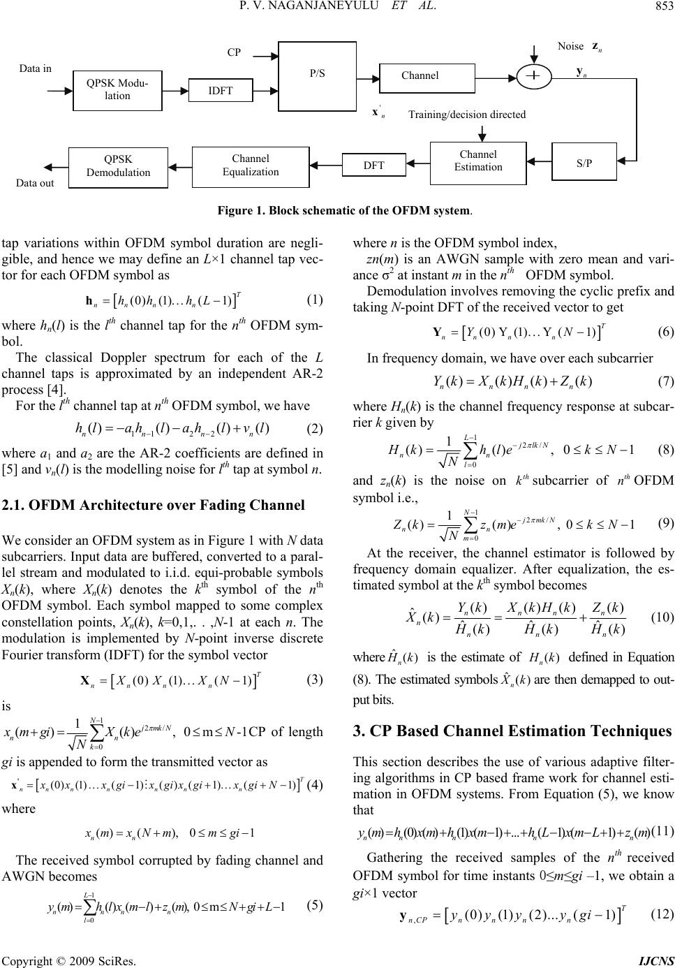 P. V. NAGANJANEYULU ET AL. 853 n Noise n z CP Figure 1. Block schematic of the OFDM system. tap variations within OFDM symbol duration are negli- gible, and hence we may define an L×1 channel tap vec- tor for each OFDM symbol as (0)(1). . . (1)T nnnn hh hLh (1) where hn(l) is the lth channel tap for the nth OFDM sym- bol. The classical Doppler spectrum for each of the L channel taps is approximated by an independent AR-2 process [4]. For the lth channel tap at nth OFDM symbol, we have 112 2 ()()() () nnn hlah l ahl vl (2) where a1 and a2 are the AR-2 coefficients are defined in [5] and vn(l) is the modelling noise for lth tap at symbol n. 2.1. OFDM Architecture over Fading Channel We consider an OFDM system as in Figure 1 with N data subcarriers. Input data are buffered, converted to a paral- lel stream and modulated to i.i.d. equi-probable symbols Xn(k), where Xn(k) denotes the kth symbol of the nth OFDM symbol. Each symbol mapped to some complex constellation points, X n(k), k=0,1,. . ,N-1 at each n. The modulation is implemented by N-point inverse discrete Fourier transform (IDFT) for the symbol vector (0) (1). . . (1)T nnn n XX XNX (3) is 1 2/ 0 1 ()(), 0m N jmkN nn k -1 x mgi XkeN N CP of length gi is appended to form the transmitted vector as (0)(1) . . . (1)()(1). . . (1)T nnnnnnn xxxgixgixgixgi N ' x (4) where ()(), 01 nn x mxNmmgi The received symbol corrupted by fading channel and AWGN becomes 1 0 ()()()(), 0m1 L nnnn l y mhlxmlzm NgiL (5) where n is the OFDM symbol index, zn(m) is an AWGN sample with zero mean and vari- ance σ2 at instant m in the nth OFDM symbol. Demodulation involves removing the cyclic prefix and taking N-point DFT of the received vector to get (0) Y(1). . . Y(1)T nn nn YNY (6) In frequency domain, we have over each subcarrier ()()()() nnnn YkXkH kZ k (7) where Hn(k) is the channel frequency response at subcar- rier k given by 1 2/ 0 1 ()(), 01 L jlkN nn l Hkhlek N N (8) and zn(k) is the noise on subcarrier of nOFDM symbol i.e., th kth 1 2/ 0 1 ()(), 01 N jmkN nn m Zkzmek N N (9) At the receiver, the channel estimator is followed by frequency domain equalizer. After equalization, the es- timated symbol at the kth symbol becomes ()()()() ˆ() ˆˆˆ ()()() nnnn n nn YkXkH kZ k Xk n H kHkH k (10) where is the estimate of ˆ() n Hk () n H k ) defined in Equation (8). The estimated symbolsˆ( n X kare then demapped to out- put bits. 3. CP Based Channel Estimation Techniques This section describes the use of various adaptive filter- ing algorithms in CP based frame work for channel esti- mation in OFDM systems. From Equation (5), we know that ()(0)() (1)(1)...(1)(1)( nn nnn ymhxmhxmhLxmLzm) (11) Gathering the received samples of the nth received OFDM symbol for time instants 0≤m≤gi –1, we obtain a gi×1 vector ,(0) (1) (2)...(1)T nCPnn nn yyy ygiy (12) n y Channel S/P Training/decision directed ' n x Data out Channel Estimation DFT Channel Equalization QPSK Demodulation Data in P/S QPSK Modu- lation IDFT Copyright © 2009 SciRes. IJCNS  P. V. NAGANJANEYULU ET AL. 854 which is the CP of the received OFDM symbol, and ,(0) (1) (2)...(1)T nCPnn nn zzz zgiz (13) is the gi×1 vector of AWGN samples affecting the CP part of the nth received OFDM symbol. 3.1. Kalman Filtering (KF) Algorithm When operating in a non-stationary environment, Kal- man filter [6] is known to yield an optimal solution to the linear filter problem. This subsection describes the ap- plication of KF to the channel estimation problem in OFDM. For this purpose, the system is formulated as a state-space model, with unknown channel taps compris- ing the state of the system. We assume that the state Sn, to be estimated at OFDM symbol index n, comprises of channel taps at two consecutive OFDM symbols [7]. 121 T nnn L shh (14) From Equation (1) and Equation (2) we have 1 (0)(1). . . (1)T nnn n L hhhL h 11111 (0)(1). . . (1)T nnnn L hh hL h and 1122nn n aa n hh hv (15) From above equations we get 12 21 nn LL L n nL1Ln aa hh 0I v hIIh (16) We observe that Equation (16) provides the basis for forming the process equation as 1nnn sBs v (17) Here, transition matrix 222 LL L L1L L L aa 0I BII (18) 0L×L denotes the L ×L matrix of all zeros and IL is the L ×L identity matrix. Process noise vector 1L 21 (0)(1)...(1) T nnnn L vv vL v0 (19) where vn(l) is the modelling noise as in (2) From Equation (11), we have ( )(0)( )(1)(1)...(1)(1)( ) nn nnn ymhxmhxmhLxmLzm 11 1 (0)(0) (1) . . . (1) (1)(1) (0) (1) . . . (1) nnnn nn nn n yx xNgixNgiL yx xxNgi ygi (0) (1) (1) (2) . . . ()(1) n n nnn n h h xgixgixgi LhL () n z m where 01mgi We observe from above that following provides the basis for forming measurement equation as ,nCPn nnCP , y As z (20) where the measurement matrix n Ain Equation (20) is formed from the matrix An by augmenting it with a null matrix as L2 ngi n g iL A0 A (21) Here A n is a gi×L matrix of transmitted symbols that determine the CP of the received OFDM symbol. 11 1 (0) (1) . . . (1) (1) (0) (1) . . . nn n nn n n xx Ngix NgiL xx xNgi A (1) (2) . . . () nn n g iL xgixgixgi L Considering that the CP appended to an OFDM sym- bol is a replication of the last gi values of that symbol, we may write An in terms of transmitted CP value as, 11 1 11 (0) (1) (2) . . . (1) (1) (0) (1) . . . (2) ( nn nn nnnn n n xxgixgi xgiL xxxgixgiL x A 1) (2) . . . () nn g iL gix gix giL An has gi rows corresponding to gi consecutive time instants of the CP. The L elements of each row are the transmitted symbol values affecting the received CP value at that instant. This matrix structure assumes that the CP length is at least equal to the number of taps in the channel impulse response, i.e. no inter block interference. The measurement noise vector Zn,CP, in Equation (20), comprises the gi×l vector of AWGN samples affecting the cyclic prefix part of the OFDM symbol. We observe that Equation (17) and Equation (20) pro- vide the basis for forming the process equation and measurement equation, respectively for the state space model, as follows 1nnn sBs v ,nCPn nnCP , y As z (22) A Kalman filter is employed to estimate the unknown Copyright © 2009 SciRes. IJCNS  P. V. NAGANJANEYULU ET AL. 855 Q state of the system. Cyclic prefix of the received OFDM symbol yn,CP is given as input observation to Kalman algorithm, the following estimation equations are given by [3] |12 21|11 [] H nnL Ln n BBPP (23) 1, 1 ˆ [] nginCP nn αyAs (24) |1 2 [] H ngigin nnn CAAPQ (25) 1 2|1 [] H nLginnn n KAPC (26) 21 1 ˆˆ [] nLn nn sBsKα (27) 1 ˆˆ [] nLn R hs , 2 [ ] L LLLL R 0I (28) 22 2|1 [] [] nLLLnnnn IKAPP (29) where Kn is the 2L×gi Kalman gain matrix , is the state estimate at the nth OFDM symbol, Q1 and Q 2 are the covariance matrices of vn and Zn,CP respectively, Pn|n-1 is the priori covariance matrix of estimation error , and Pn is the current covariance matrix of estimation error. When the channel taps are modelled as a zero mean random process, the algorithm is initialized with an all-zero state vector. Besides this, the assumption of un- correlated scattering (US) causes the different channel taps to be i.i.d., and the error covariance matrix is ini- tialized as an identity matrix. ˆn s 00 2 ˆ1 L ss0 00000 ˆˆ ()() H n E ssssIP The receiver operates in training and decision directed modes. In training mode the known transmitted CP (xn,CP ) and CP part of the received OFDM symbol (yn,CP) form the input to the above Kalman filter algorithm, and get the channel estimation Hn(k), we get () ˆ() ˆ() n n n Yk Xk H k (30) In decision directed mode the receiver uses the esti- mated channel vector from the previous OFDM symbol to demodulate the received symbol and generate an esti- mate of transmitted CP (). Here the transmitted CP part can be estimated by previous estimated channel i.e., , ˆ() nCP Xk , , 1 () ˆ() ˆ() nCP nCP n Yk Xk Hk (31) This estimated CP and CP of the received OFDM symbol (yn,CP) helps to estimate the channel. The equations from (23) to (29) can be carried out by providing the AR parameters that are involved in the transition matrix B and the driving process variances are available. In case, these are unknown, for estimating these parameters Dual-Kalman filtering technique is used. 3.2. Dual-Kalman Filtering Algorithm To estimate the AR parameters θn from the estimated fading process ĥn, Equation (28) is firstly represented as an AR-2 model to express the estimated fading process as a function of θn (AR parameter vector). 1 12 2 ˆˆˆ nnn a a hhhw n n (32) 12 1 12 221 12 12 ˆˆˆ (0)(0) (0) ˆˆˆ (1)(1) (1) ˆˆˆ (1)(1) (1) nnn nnn n nnn LL hhh a hhh a hLh LhL w nn rHθw (33) where rn is the estimated channel vector, θn is the AR parameter vector defines as . 12 [ ] T naaθ and wn is the L×1 noise vector as in Equation (19). When the channel is assumed to be stationary, the AR parameters are time-invariant and satisfy the following relationship 1nn θθ (34) As Equation (33) and Equation (34) define a state- space representation for the estimation of the AR pa- rameters, a second Kalman filter can be used to recur- sively estimate θn as follows [3] /1 1/1 22 [] nnn n PP (35) 1 ˆ [] [ nLnn αrHθ1 ] (36) /1 3 [] nnn H LL CHHPQ n C (37) /1 1 2 [] nnn H L KHP (38) 21 1 ˆˆ [] nn nn θθKα (39) // 22 2 [] [] nnn nn 1 IKHPP (40) where Q3 is the covariance matrix of the wn , the error covariance matrix and the initial AR parameter vector are defined as 002 ˆ θθ01 2 0/0 0000 ˆˆ ()() H E θθθθ IP 3.3. Noise parameters estimation Apart from estimating the AR parameters, we also need to estimate the noise parameters for the fading channel Copyright © 2009 SciRes. IJCNS  P. V. NAGANJANEYULU ET AL. Copyright © 2009 SciRes. IJCNS 856 4. Results and Conclusions In this analysis we compare CP based dual Kalman and Kalman. At SNR of 10db, BER of Kalmanis 10-0.8 where as for dual Kalman; this value is 10-1.81. For Overall SNR is concerned, dual Kalmangives better performance and doesn’t require any additional training sequence like training bits and noise. (Figure 2) 5. References [1] R. Steele, “Mobile radio communications,” New York: IEEE Press, 1992. [2] X. W. Wang and K. J. R. Liu, “Adaptive channel estimation using cyclic prefix in multicarrier system,” IEEE Commu- nication Letters Magazines, Vol. 3, pp. 291–293, October 1999. Figure 2. BER v/s SNR for Kalman and Dual Kalman. environment i.e., variance of v n and Zn,CP. This can be done by using the error covariance matrices. From Equa- tion (23) and Equation (29) we can write the noise vari- ances recursively as [3] A. Jamoos, D. Labarre, E. Grivel, and Najim, “Two cross coupled Kalman filters for joint estimation of MC-DS- CDMA fading channels and their corresponding autore- gressive parameters,” Proceedings of EUSIPCO, Antalya, Turkey, September 4–8, 2005. 22 1|1 [] H HH nLLnn nnnnn BBKααKLPP (41) [4] M. K. Tsatsanis, G. B. Giannakis, and G. Zhou, “Estimation and equalization of fading channels with random coeffi- cients,” Signal Process, Vol. 53, pp. 211–229, 1996. 11 11 ˆˆ ()( 1)T n n Qn Qn nn D LD (42) 12 1 0 . . . . . 0 L D [5] A. Jamoos, J. Grolleau, and E. Grivel, “Kalman vs H∞ algo- rithms for MC-DS-CDMA channel estimation with or with- out a priori AR modelling,” IEEE Multicarrier Spread Spectrum, Springer Verlag, pp. 427–436, 2007. |1 [] H H ngigin nn nnn Mαα AAP (43) 221 11 ˆˆ ()( 1)T n n Qn Qn nn M[6] I. R. Petersen and A. V. Savkin, “Robust Kalman filtering for signals and systems with large uncertainties,” Boston, MA: Birkhäuser, 1999. 1 D D (44) 11 1 0 . . . . . 0 g i D, [7] Y. Li, L. J. Cimini, and N. R. Sollenberger, “Robust chan- nel estimation for OFDM systems with rapid dispersive fading channels,” IEEE Transactions on Communications, Vol. 46, pp. 902–915, July 1998. where and are the estimated variances of the process noise vn and modelling noise Zn,CP respec- tively. 1 ˆ()Qn 2 ˆ()Qn |