Int. J. Communications, Network and System Sciences, 2009, 2, 836-844
doi:10.4236/ijcns.2009.29097 Published Online December 2009 (http://www.SciRP.org/journal/ijcns/).
Performance Analysis of an Optimal Circular
16-QAM for Wavelet Based OFDM Systems
Khaizuran ABDULLAH, Seedahmed S. MAHMOUD*, Zahir M. HUSSAIN
School of Electrical & Computer Engineering, RMIT University, Melbourne, Australia
*Future Fiber Technologies Pty. Ltd., Mulgrave, Australia
Received August 20, 2009; revised September 29, 2009; accepted October 29, 2009
Abstract
The BER performance for an optimal circular 16-QAM constellation is theoretically derived and applied in
wavelet based OFDM system in additive white Gaussian noise channel. Signal point constellations have been
discussed in much literature. An optimal circular 16-QAM is developed. The calculation of the BER is based
on the four types of the decision boundaries. Each decision boundary is determined based on the space dis-
tance d following the pdf Gaussian distribution with respect to the in-phase and quadrature components nI
and nQ with the assumption that they are statistically independent to each other. The BER analysis for other
circular M-ary QAM is also analyzed. The system is then applied to wavelet based OFDM. The wavelet
transform is considered because it offers a better spectral containment feature compared to conventional
OFDM using Fourier transform. The circular schemes are slightly better than the square schemes in most
SNR values. All simulation results have met the theoretical calculations. When applying to wavelet based
OFDM, the circular modulation scheme has also performed slightly less errors as compared to the square
modulation scheme.
Keywords: Performance OFDM, Fourier-Based OFDM, Wavelet-Based OFDM, Circular 16-QAM, Square
16-QAM
1. Introduction
Quadrature amplitude modulation (QAM) is one of the
most popular modulation schemes used by orthogonal
frequency division multiplexing. Some popular types of
M-ary QAM are 4-QAM, 16-QAM and 64-QAM. The
number of 4, 16 and 64 is corresponding to 22, 24 and 26
in which that the superscript number 2, 4 or 6 is the bit
rate per OFDM symbol respectively. In this paper, the
constellation points derivation and the BER analysis are
focused on 16-QAM, which gives an intermediate result
of BER performance between 4- and 64-QAM in an
AWGN channel [1]. The 16-QAM is also one of the
standard modulation schemes in OFDMs’ applications
such as terrestrial Digital Video Broadcasting (DVB),
Digital Audio Broadcasting (DAB) and High Perform-
ance Radio LAN Version 2 (HIPERLAN/2) [2]. In the
transmitter, an OFDM symbol is mapped from binary to
complex signal with amplitude and phase represented in
real and imaginary number. On the other hand, the signal
is demapped or extracted from complex signal to OFDM
symbol in the receiver. The decision boundary is needed
to detect the correct symbols between the transmitter and
receiver. The bit error rate (BER) performance is deter-
mined after performing the difference of errors between
the transmitted bits with the received bits. The BER per-
formance of M-ary QAM has been investigated by sev-
eral authors. The exact BER expressions for QAM is
presented in [3]. An extension of BER expressions con-
sidering of an arbitrary constellation size is discussed in
[4]. Both works include the square constellation points.
In this paper, we propose an alternative BER expres-
sion using optimal circular constellation points. The cal-
culation of probability of error is based on determining
the decision boundary. We have proposed four types of
decision boundaries.
Based on these types, the probability of error occurs
when the receiver is making an incorrect decision. To the
best of our knowledge, there is no work of the probabil-
ity of error calculation for a circular 16-QAM with the
application of wavelet-based OFDM, namely discrete
wavelet transform (DWT). The principle feature of DWT
is it has low pass and high pass filters satisfying perfect
reconstruction property in the transmitter and receiver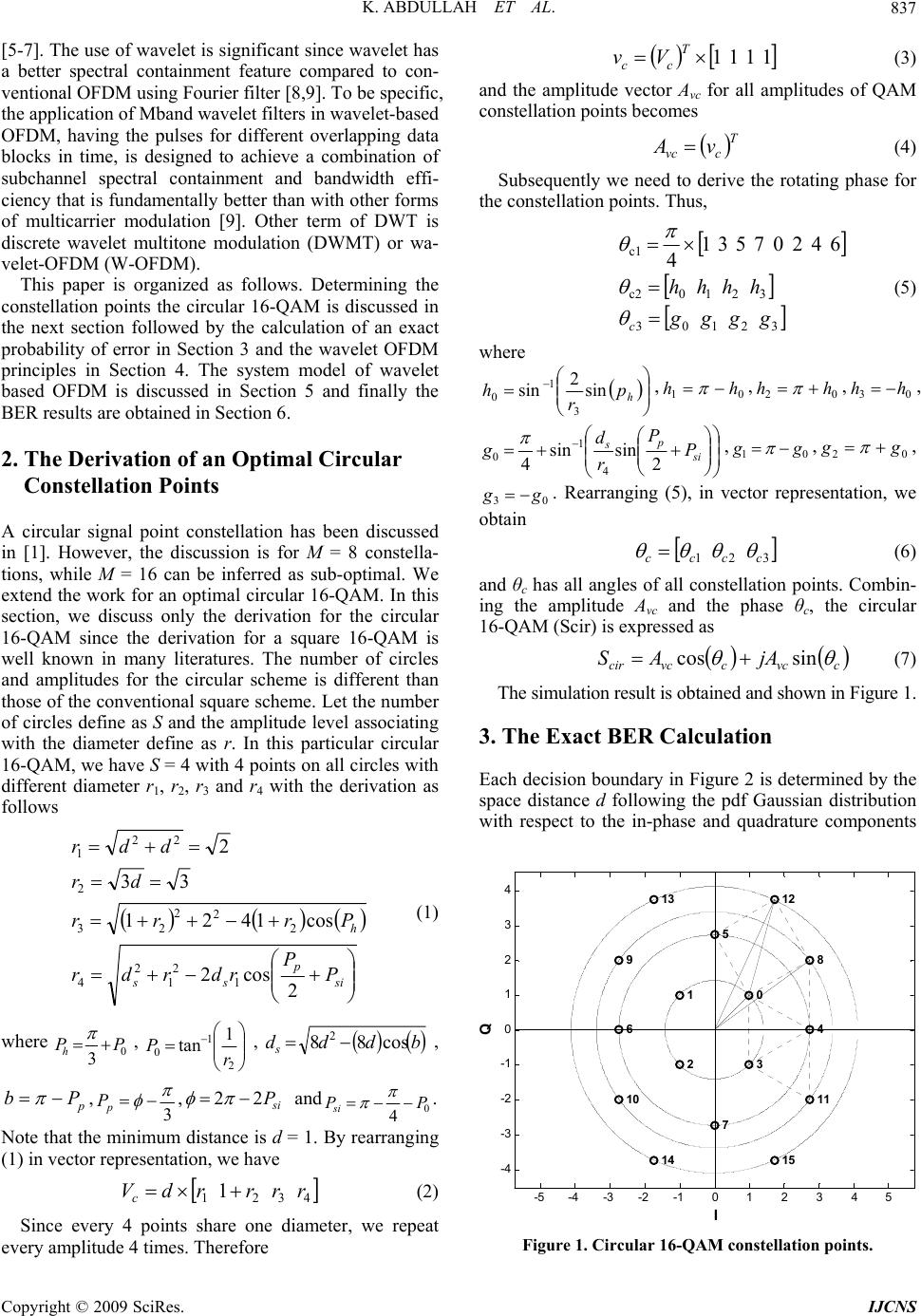

K. ABDULLAH ET AL. 837
[5-7]. The use of wavelet is significant since wavelet has
a better spectral containment feature compared to con-
ventional OFDM using Fourier filter [8,9]. To be specific,
the application of Mband wavelet filters in wavelet-based
OFDM, having the pulses for different overlapping data
blocks in time, is designed to achieve a combination of
subchannel spectral containment and bandwidth effi-
ciency that is fundamentally better than with other forms
of multicarrier modulation [9]. Other term of DWT is
discrete wavelet multitone modulation (DWMT) or wa-
velet-OFDM (W-OFDM).
This paper is organized as follows. Determining the
constellation points the circular 16-QAM is discussed in
the next section followed by the calculation of an exact
probability of error in Section 3 and the wavelet OFDM
principles in Section 4. The system model of wavelet
based OFDM is discussed in Section 5 and finally the
BER results are obtained in Section 6.
2. The Derivation of an Optimal Circular
Constellation Points
A circular signal point constellation has been discussed
in [1]. However, the discussion is for M = 8 constella-
tions, while M = 16 can be inferred as sub-optimal. We
extend the work for an optimal circular 16-QAM. In this
section, we discuss only the derivation for the circular
16-QAM since the derivation for a square 16-QAM is
well known in many literatures. The number of circles
and amplitudes for the circular scheme is different than
those of the conventional square scheme. Let the number
of circles define as S and the amplitude level associating
with the diameter define as r. In this particular circular
16-QAM, we have S = 4 with 4 points on all circles with
different diameter r1, r2, r3 and r4 with the derivation as
follows
 











si
p
ss
h
P
P
rdrdr
Prrr
dr
ddr
2
cos2
cos1421
33
2
1
2
1
2
4
2
2
2
23
2
22
1
(1)
where 0
3PP
h

,








2
1
0
1
tan r P,
  bdddscos88 2 ,
p
Pb 

,
3

 
p
P,si
P22




and0
4PP
si 


.
Note that the minimum distance is d = 1. By rearranging
(1) in vector representation, we have

4321 1rrrrdVc


 (2)
Since every 4 points share one diameter, we repeat
every amplitude 4 times. Therefore

  1111 T
cc Vv
 (3)
and the amplitude vector Avc for all amplitudes of QAM
constellation points becomes

T
cvcvA  (4)
Subsequently we need to derive the rotating phase for
the constellation points. Thus,



32103
3210c2
c1 64207531
4
gggg
hhhh
c






(5)
where










h
p
r
hsin
2
sin
3
1
0,01hh 


,02 hh 

,03hh


,








si
pP
P
21
g








 s
r
d
gsinsin
44
1
0

, ,
0
g 
2
g0 g



,
03 gg


. Rearranging (5), in vector representation, we
obtain


321cccc





(6)
and θc has all angles of all constellation points. Combin-
ing the amplitude Avc and the phase θc, the circular
16-QAM (Scir) is expressed as
 
cvccvccir jAAS


sincos

(7)
The simulation result is obtained and shown in Figure 1.
3. The Exact BER Calculation
Each decision boundary in Figure 2 is determined by the
space distance d following the pdf Gaussian distribution
with respect to the in-phase and quadrature components
-5 -4 -3 -2 -1 0 1234 5
-4
-3
-2
-1
0
1
2
3
4
0 1
2 3
4
5
6
7
8 9
10 11
12 13
14 15
I
Q
Figure 1. Circular 16-QAM constellation points.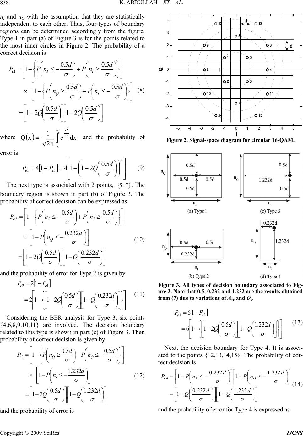

K. ABDULLAH ET AL. 838
nI and nQ with the assumption that they are statistically
independent to each other. Thus, four types of boundary
regions can be determined accordingly from the figure.
Type 1 in part (a) of Figure 3 is for the points related to
the most inner circles in Figure 2. The probability of a
correct decision is









































































d
Q
d
Q
d
nP
d
nP
d
nP
d
nPP
IQ
IIc
5.0
21
5.0
21
5.05.0
1
5.05.0
1
1
(8)
where




x
2
x
dxe
2π
1
xQ
2
and the probability of
error is























2
11
5.0
211414

d
QPP ce (9)
The next type is associated with 2 points,


75,. The
boundary region is shown in part (b) of Figure 3. The
probability of correct decision can be expressed as





























































d
Q
d
Q
d
nP
d
nP
d
nPP
Q
IIc
232.0
1
5.0
21
232.0
1
5.05.0
1
2
(10)
and the probability of error for Type 2 is given by








































d
Q
d
Q
PP ce
232.0
1
5.0
2112
12 12
(11)
Considering the BER analysis for Type 3, six points
{4,6,8,9,1 0,11} are involved. The decision boundary
related to this type is shown in part (c) of Figure 3. Then
probability of correct decision is given by





























































d
Q
d
Q
d
nP
d
nP
d
nPP
I
QQc
232.1
1
5.0
21
232.1
1
5.05.0
1
3
(12)
and the probability of error is
-5 -4 -3 -2 -1012 345
-4
-3
-2
-1
0
1
2
3
4
0 1
2 3
4
5
6
7
8 9
10 11
12 13
14 15
I
Q
d
d
Figure 2. Signal-space diagram for circular 16-QAM.
Figure 3. All types of decision boundary associated to Fig-
ure 2. Note that 0.5, 0.232 and 1.232 are the results obtained
from (7) due to variations of Avc and Өc.










































d
Q
d
Q
PP ce
232.1
1
5.0
2116
16 33
(13)
Next, the decision boundary for Type 4. It is associ-
ated to the points {12,13,14,15}. The probability of cor-
rect decision is
















































d
Q
d
Q
d
nP
d
nPPQIc
232.1
1
232.0
1
232.1
1
232.0
1
4
(14)
and the probability of error for Type 4 is expressed as

K. ABDULLAH ET AL. 839








































d
Q
d
Q
PPce
232.1
1
232.0
114
14 44
(15)
Combining and rearranging Equations (9), (11), (13)
and (15), the average probability of error for the circular
16-QAM scheme is given by





















CCBCBAA
PPPPPeeeecir
5
2
3
23
4
1
28
8
1
16
1
4321
(16)
where 





σ
0.5d
QA ,





σ
0.232d
QB and






σ
1.232d
QC . Using
 1M2
M.E3log
db2

from [4]
where M=16 and 5
N
2
1
σ0 , Equation (16) can be
expressed as in term of energy per bit over noise density
ratio 







0
b
N
E.
Thus parameters A, B and C can be rewritten as
 γ0.5QA , 

 γ0.232QB
and
 γ1.232QC where
0
2
1
4N
Eb
 
.
The analysis can also determine the exact BER for
other circular M-ary QAM. Note that the process of ob-
taining BER analysis for the square scheme is excluded
since it is available in much literature.
4. Wavelet OFDM Principles
A wavelet is normally assigned the square integrable
function ψ(t) to illustrate the wavelet fundamental
definition [10]. In other literature [7], it is also indicated
by ψ(t) where L is a Lebesque integral and 2
signifies the integral of the square of the modulus of the
function, and R denotes the real number for integration
of the independent variable t. In this section, we discuss
two principles of wavelet transforms, orthogonal and
biorthogonal wavelet as follows.

RL2 
4.1. Orthogonal Wavelets
The Fourier transform has exponential parts consisting of
cosine and sine signal bases. These bases are orthogonal
to each other. The wavelet transform also has orthogonal
bases. Its bases are low pass and high pass filters which
are associated with the scaling and wavelet functions
respectively. Among orthogonal wavelets are Daube-
chies, Coiflets, Morlet and Meyer [6].
Orthogonal wavelet functions can be generated by
scaling and shifting properties as follows [10]:







a
bt
t
ab

2
1 (17)
where a and b are the scaling and shifting real parameter
values. According to [11], the wavelet transform is called
continuous if a and b are continuous. The drawbacks of a
continuous wavelet transform are redundancy and im-
practicality. To avoid these problems, those parameters
have to be discredited as follows [10,12]:
anbb
aa m
0
0

 (18)
where m and n indicates the exponential integers. From
(17) and (18), the basis of the DWT can be formed as
  (19)
00
2
0nbtaat m
m
mn  


Using a0 = 2 and b0 = 1, we can have the signal func-
tion
 













L
mn
m
m
mn
n
L
nL
ntD
ntCtU
1
2
,
22
2


(20)
where the scaling coefficient CL.n is


 



dtnttU
ttUC
L
L
nLnL
22
,
2
,.


(21)
where   nttL
L
 
222
nL,
  and the wavelet coeffi-
cient Dmn is


 



dtnttU
ttUD
L
L
mnmn
22
,
2


(22)
In (20), the time domain signal U(t) is DWT trans-
formed to scales in which all the coefficients are denoted
as the scales [10]. U(t) can also be called the finite resolu-
tion wavelet representation [12]. The sum of scaled φ(2t)
can make up the parent scaling function, and can be ex-
pressed as [7,10]:




n
nntht 22

(23)

K. ABDULLAH ET AL. 840
where the coefficients hn are a sequence of real or perhaps
complex numbers called the scaling function (or scaling
vector or filter). The use of 2 is to maintain the norm
of the scaling function with the scale of 2. This scaling
function in (23) can also be used for the multiresolution
analysis (MMRA) [13]. A fundamental wavelet function
can be expressed as a linear combination of translates of
the scaling function as follows [10,12]:
 

n
nntgt 22
 
(24)
where the wavelet coefficients gn are related to the scaling
coefficients hn by
 
n
nhng
 1 1 (25)
An example of the application of (23) is the Haar
scaling function which is given by [7] as follows:
 122 

ttt
H



(26)
It can be seen that  t2

can be used to construct
 t
H

. It also can be noted that (26) is the result of (23)
for the first 2 sequence of discrete samples of n with co-
efficients

2
1
0h ,

2
1
1h  [7]. Examples of Haar
scaling and wavelet functions are shown in Figure 4.
The Haar wavelet can be categorised as an orthogonal
wavelet. All Daubechies wavelet families are categorised
as orthogonal wavelets [6]. Another figure of a Daube-
chie wavelet such as db2 is shown in Figure 5.
4.2. Biorthogonal Wavelets
Biorthogonal wavelets are different than orthogonal
wavelets because they have biorthogonal bases. Their
bases have symmetric perfect reconstruction properties
with compactly support. They also have two duality
functions for each scaling and wavelet functions which
are

and for the scaling filters, and ψ and

ˆ

ˆ
for the wavelet filters accordingly. In MATLAB, we
have built-in functions such as bior1.1, bior2.2, bior5.5,
rbio1.1, rbio2.2 and rbio5.5. The number next to the
wavelet name refers to the length of the filter in the de-
composition and reconstruction filters respectively.
Biorthogonal wavelets can be constructed from or-
thogonal wavelets by considering the duality concept.
Let

and be two scaling functions and let ψ and 
ˆ

ˆbe two wavelet functions, then we can express the
biorthogonal scaling and wavelet functions as follows
[5,14]:
 
 
 
  0,
ˆ
0
ˆ
,
ˆ
,
ˆ
,




ntt
tt
tt
tt
k
n




(27)
where






n
nntht 2
ˆ
ˆ
2
ˆ

and




n
nntht 2
ˆ
ˆ
2
ˆ

with n

and k

are the results of biorthogonal bases.
The last two equations in (27) satisfy the orthogonality
properties. One advantage of using biorthogonal wave-
lets is that the scaling and wavelet functions are symmet-
ric due to the duality concept [5,7], therefore, biorthogo-
nal wavelets provide an advantage over orthogonal
-0.5 00.5 11.5
-1
-0. 8
-0. 6
-0. 4
-0. 2
0
0.2
0.4
0.6
0.8
1
-0.5 00.5 11.5
-1
-0.8
-0.6
-0.4
-0.2
0
0.2
0.4
0.6
0.8
1
Figure 4. Haar (db1) scaling function (left) and wave-
let function
 t 


t  (right).
Figure 5. Db2 scaling function (left) and wavelet func-
tion
 t 

 t  (right). Note that this plot is similar to [5] p. 197
and [7] p. 81.

K. ABDULLAH ET AL. 841
05 10
-1.5
-1
-0.5
0
0.5
1
1.5
2

'
05 10
-1.5
-1
-0.5
0
0.5
1
1.5
2

Figure 6. Bior5.5 shows duality concept with two scaling
functions, (left) and 
ˆ

(right). Note that this plot is
similar to [5] p. 280.
Figure 7. Bior5.5 shows duality concept with two wavelet
functions, (left) and (right). Note that this plot
is similar to [5] p. 280.
 t 
ˆ

t 
wavelets because they offer not only orthogonality but
also symmetry. In [15], comparing orthogonal transforms,
biorthogonal transforms relax some of the constraints on
the mother wavelet (or filters) and allow the mother
wavelet to be symmetric and have linear phase. The plots
of biorthogonal scaling and wavelet functions are shown
in Figure 6 and Figure 7.
5. System Model of Wavelet-Based OFDM
The wavelet transform blocks comprise of an inverse
discrete wavelet transform (IDWT) at the transmitter and
a discrete wavelet transform (DWT) at the receiver as
shown in Figure 8. Due to the overlapping nature of
wavelets, the wavelet-based OFDM does not need a cy-
clic prefix to deal with the delay spreads of the channel.
As a result, it has a higher spectral containment than in
Fourier based OFDM [8,9]. The DWT-OFDM system
model comprise of low pass as LPF filter coefficients
and h as HPF filter coefficients, the orthonormal bases
are satisfied by four possible ways as follows [6]:
1, *gg (28)
1, *hh (29)
0,*hg (30)
1, *gh (31)
where (28) or (29) is related to the normal property and
(30) or (31) is for orthogonal property accordingly. The
commas and star symbols in Equations (28) to (31)
above are referring to the dot product and transpose vec-
tor accordingly. Both filters are assumed having perfect
reconstruction property. This means that the input and
output of the two filters are expected to be the same. The
g and h coefficients can be further described as having
convolution operations to perform as orthonormal wave-
lets which can be represented as [16]
 

 ng
n
g
n
g
n
gn
ng
n
g
n
g
n
hn
ji
NN
N
jiii
i
*...*
2
*...
...*
2
*
2
*...*
2
*...*
2
*
2
12
1












































(32)
where

 ji

is a positive integer for N-2. ,...,1,0, ji
The signal is up-sampled and filtered by the LPF coef-
ficients or namely as approximated coefficients.
The system model in Figure 8 is assumed that there is
no frequency offset so that the DWT itself acts as a
matched filter at the receiver. To determine the data in
sub-channel k, we match the transmitted waveform with
carrier i [17]:
Figure 8. The system model of wavelet based OFDM transceiver.

K. ABDULLAH ET AL. 842
  




1
0
,,
N
k
ikki tWtWdWty (33)
where y(t) is the transmitted data via IDWT, dk is the
data projected onto each carrier, Wk(t) are the com-
plex exponentials or it can be written as N
m
j2π2
e,
  tWtW ik , equals 1 when k = i and 0 when ik

.
In a typical communication system, data is transmitted
over a dispersive channel. The impulse response of a
deterministic (and possibly time-varying) channel can be
modeled by a linear filter h(t):









1
11
''
,
000
*
g
NN
kk klk
klk
rtyt htnt
dWdWtlknt




 


(34)
where , and g (g > 1) is the wavelet
genus so that Ng is the filter order (number of taps in that
subband), and n(t) is an additive white Gaussian noise.
Due to the overlapped nature of the wavelet-based
OFDM, it requires g symbol periods, for a genus g sys-
tem, to decode one data vector [17]. This is the reason of
having the wavelet transforms of g-1 other data vectors
in the second term of (34).
  thtWk*W'
k
After matched-filtering with carrier i, the signal be-
comes
  

 
 
 
 
1
'
0
1
'
,
0
1
1
,0
0
1
,,
0
1
,,
10
,,
,
,
0,
00
"
N
ikki
k
N
gkl ki
k
l
i
N
kk i
k
N
kii kki
k
ki
gN
kl ki
lk
ki
rtW tdWtW t
d WtlkWtlk
ntft
dntft
dd
dlnt





























(35)
where  0
,iik
d

is the recovered data with correlation
term  0
,ii

. The second term which is
is the interference due to the distorted filters that are no
longer orthogonal to one another with correlation terms




1
,0
,0
N
ikk
ikk
d 
 0 
,ik

, and is the interference term
with correlation




N
ikk
iklk ld
1
,0
,,

 l
ik ,

g
l1

due to the overlapped nature of
the wavelet transform. If the channel has no distortion,
only the first and last terms would appear, which result
that the decoder would obtain almost the correct signal.
6. System Performance
The performance between the square and circular for
16-QAM for unfiltered constellation points is discussed
in Subsection 6.1. A filtered version, which is the proc-
essed signal through the matched filter and DWT block
shown in Figure 8 at the receiver, is then considered. The
result is obtained and discussed in Subsection 6.2.
6.1. Square versus Circular
In this subsection, two main parts are discussed. The first
part is to obtain the simulation result for circular 16-
QAM from (16) and compare with the square 16-QAM
provided by (17) in [4] which is written as follows
 


 

2
0
2
2
0
2
3log.
1
21
log
3log .
2
21
log
b
sq
b
ME
M
PQ
MN
MM
ME
MQMN
MM












(36)
Note that the square 16-QAM curve in Figure 9 is also
approximately similar to the theoretical 16-QAM plot if
one uses the Bit Error Rate Analysis Tool (bertool) from
Matlab. From the figure, it is shown that the circular
scheme slightly outperforms the counterpart scheme at
most SNR values.
The second part is to obtain the result for other M-ary
QAM. The exact BER analysis for other circular M-ary
QAM is performed by changing the value of M in
 1M2
M.E3log
db2

 and fix σ accordingly. When M is
changed, the parameters A, B and C are consequently
affected. Then, they are substituted into (16). Table I
shows the summary of the arbitrary parameters due to
varying M. Figure 9 also shows the BER results for other
circular schemes with comparisons of other square QAM.
The circular of other M-ary QAM are also slightly better
than the square schemes in most SNR values. The simu-
lation results show that they met the theoretical analysis.
6.2. Wavelet Based OFDM
To simulate the system using wavelet based OFDM (W-OF-
DM), the orthogonal wavelet family such as Daubechies,

K. ABDULLAH ET AL. 843
Figure 9. Exact BER of circular and square M-ary QAM.
Figure 10. Comparison of circular and square of 16-QAM wavelet (db2 and bior5.5) and Fourier based OFDM.
db2 with comparison of the biorthogonal wavelet family,
bior5.5 are considered. From Figure 10, it is shown that
circular 16-QAM has better outperformed the square
scheme in most SNR values. It is interesting to observe
that the W-OFDMs results have less BER performance
compared to Pcir and Psq. The result is the effect of the
filtered version that have been through the imperfect
functional components in the receiver such as distorted
filters and an additive white Gaussian noise channel as
indicated in the previous section.

K. ABDULLAH ET AL. 844
Table 1. Summary of parameters for circular M-Ary (M ≤
16) Qam.
M=4 M=8 M=16
d b
E b E
14
9 b
E
5
2
γ 0
52N
Eb
0
14
45
2N
Eb
0
22 N
Eb
A 







0
5N
E
Qb








0
14
45
N
E
Qb 







0
2N
E
Qb
B 







0
5N
E
bQ b








0
14
45
N
E
bQ b








0
2N
E
bQ b
C 







0
5N
E
cQ b 







0
14
45
N
E
cQ b 







0
2N
E
cQ b
Note: b=0.464, c=2.464 and Q(.)=erfc(.)
7. Conclusions
The optimal circular 16-QAM constellation points and
the analysis of its exact BER calculation have been de-
rived. The work has also been applied to wavelet based
OFDM systems to compare the circular and square
schemes. The results showed that the circular were
slightly better than the square counterparts. When apply-
ing wavelet based OFDM using different wavelet fami-
lies (orthogonal and biorthogonal), the same results were
also obtained that the circular has slightly outperformed
the square.
8. References
[1] J. G. Proakis, “Digital communications,” Fourth edition,
New York: McGraw-Hill, 2001.
[2] R. V. Nee and R. Prasad, “OFDM for wireless multime-
dia communications,” Boston: Artech House, 2000.
[3] M. P. Fitz and J. P. Seymour, “On the bit error probabil-
ity of QAM modulation,” International Journal of Wire-
less Information Networks, Vol. 1, No. 2, pp. 131–139,
1994.
[4] K. Cho and D. Yoon, “On the general BER expression of
one and two dimensional amplitude modulations,” IEEE
Transactions on Communications, Vol. 50, No. 7, pp.
1074–1080, July 2002.
[5] I. Daubechies, “Ten lectures on wavelets,” Philapdelphia:
Society for Industrial and Applied Mathematics, 1992.
[6] M. Weeks, “Digital signal processing using matlab and
wavelets,” Infinity Science Press LLC, 2007.
[7] C. S. Burrus, R. A. Gopinath, and H. Guo, “Introduction
to wavelets and wavelet transforms,” Upper Sadle River,
NJ: Prentice-Hall, 1998.
[8] R. Mirghani and M. Ghavami, “Comparison between wa-
velet-based and Fourier-based multicarrier UWB sys-
tems,” IET Communications, Vol. 2, No. 2, pp. 353–358,
2008.
[9] S. D. Sandberg and M. A. Tzannes, “Overlapped discrete
multitone modulation for high speed copper wire com-
munications,” IEEE Journal on Selected Areas in Com-
munications, Vol. 13, No. 9, pp. 1571–1585, 1995.
[10] F. Xiong, “Digital modulation techniques,” Second edi-
tion, Boston: Artech House, 2006.
[11] I. Daubechies, “Orthonormal bases of compactly sup-
ported wavelets,” Communications in Pure and Applied
Math., Vol. 41, pp. 909–996, 1988.
[12] A. N. Akansu, “Wavelets and filter banks: A signal proc-
essing perspective,” Tutorial in Circuit and Devices, No-
vember 1994.
[13] L. Cui, B. Zhai, and T. Zhang, “Existence and design of
biorthogonal matrix-valued wavelets,” Nonlinear Analy-
sis: Real World Applications, Vol. 10, pp. 2679–2687,
2009.
[14] R. M. Rao and A. S. Bopardikar, “Wavelet transforms:
Introduction to theory and applications,” MA: Addison-
Wesley, 1998.
[15] R. K. Young, “Wavelet theory and its applictions,” Mas-
sachusetts: Kluwer Academic, 1993.
[16] B. G. Negash and H. Nikookar, “Wavelet based OFDM
for wireless channels,” Vehicular Technology Conference,
2001.
[17] N. Ahmed, ”Joint detection strategies for orthogonal fre-
quency division multiplexing,” Dissertation for Master of
Science, Rice University, Houston, Texas, pp. 1–51,
April 2000.