iBusiness, 2009, 1: 85-98
doi:10.4236/ib.2009.12012 Published Online December 2009 (http://www.SciRP.org/journal/ib)
85
A Multivariate Poisson Model of Consumer Choice
in a Multi-Airport Region
Andrew J. BUCK*, Erwin A. BLACKSTONE, Simon HAKIM
Department of Economics, Temple University, Philadelphia, USA;
*Corresponding Author.
Received August 30, 2009; revised October 3, 2009; accepted November 17, 2009
ABSTRACT
Using the results of a uniqu e telephone survey th e frequency of cons umer flights from airports in a multi-airport reg ion
are modeled using a multivariate Poisson framework, the parameters of which were estimated using a latent variable
application of the expectation maximization algorithm. This offers a different perspective since other work on airport
choice uses the results of airport intercept surveys that capture only a single choice per respondent, whereas the data
from the phone survey is count data for the airports in the study. An airport’s own-distance had the expected negative
impact on mean usage of the airport, although the cross effects were somewhat mixed. Ticket price differences between
airports were not always statistically significant. Mean usage was found to be increasing in income for PHL, but was
decreasing for the other airports, reflecting the increasing value of respondents’ time as their income rises. If the des-
tination of flights is domestic (international) then the result is to increase usage of PHL, BWI and EWR (JFK). Except
for JFK, if the purpose of travel is mostly p leasure then it results in mo re travel from JFK a nd less from the other th ree
airports. The availability of a low cost carrier wou ld result in more frequent travel.
Keywords: Airport Choice, Poisson Regression, Expectation Maximization
1. Introduction
Using the results of a unique telephone survey the fre-
quency of consumer flights from airports in a multi-air-
port region are modeled using a multivariate Poisson
framework. This offers a different perspective from pre-
vious research in two important ways. First, other work
on airport choice uses the results of airport intercept sur-
veys that capture only a single choice per respondent,
whereas the data from the phone survey used in this pa-
per is count data for the four airports in the study. Second,
models based on intercept surveys uniformly use binary
choice models such as either probit or logit methods to
estimate the model parameters of the mutually exclusive
choices [1–3]. The consumers in the present study are
observed to choose from among four airports on a re-
peated basis, resulting in a n-tuple of count data.
Modeling count data requires use of Poisson or nega-
tive binomial specifications. The present study expands
the usual statistical count model to the appropriaten-tuple
count model in the form of the multivariate Poisson so
that the counts can have non-zero covariances. The fun-
damental difference between earlier work and that pre-
sented here is the difference between allocation modeling
and modeling at the extensive margin. Until recently the
use of multivariate Poisson regression was not an option
[4]. An expectation maximization algorithm is used to
estimate the parameters of a multivariate Poisson model
of consumer decisions.
Until 1983 the Civil Aeronautics Board (CAB) was
responsible for regulating airfares in the United States.
As a consequence of that regulation commercial passen-
ger carriers competed on many dimensions other than
price. Such behavior was recognized as being economi-
cally inefficient: the price system was not being allowed
to direct resources to their greatest value in use. The
CAB was dismantled on the premise that price competi-
tion among carriers would benefit consumers and direct
productive resources to their greatest value in use. It was
felt that, inter alia, the threat of entry would be sufficient
to prevent airlines from being able to exploit apparent
monopoly power. That premise ignores the fact that
consumers are an essential element in the exercise of
market power. If consumers do not search for low fares
or fare differences are unimportant, then it is unlikely
that the threat of entry will have much impact on the fare
structure: The effect of the entry of a low fare carrier will
only be the reallocation of fliers among carriers at an

A Multivariate Poisson Model of Consumer Choice in a Multi-Airport Region 86
airport, with little impact on the allocation of passengers
among airports. Indeed, one of the current stylized facts
about air travel is that there is more variation in price
among carriers at an airport than among airports. It is
possible to evaluate the effect of low fares on consumer
behavior, and by implication the likely success of the
threat of entry as a disciplinary device, by examining
multi-airport markets. The unwillingness of flyers to
travel to other airports to obtain lower fares increases the
ability of carriers to exploit monopoly power and dis-
criminate in prices1. Since broad geographic markets are
often used in merger cases2 our analysis may shed some
light on such markets.
Heretofore airport choice studies have focused on the
choice of airport for a particular trip using intercept sur-
veys of travelers in the chosen airport. Ashford and
Benchemam [5] studied airport choice in central England
for the period 1975–1978. Among business travelers dis-
tance to the airport was the most important variable, fol-
lowed by frequency of service. Fare was found to be
most important among those traveling for pleasure.
Caves et al. [6] found that access time, frequency and
fare to be significant variables in a model of choice be-
tween mature and emerging airports in England.
Thompson and Caves [7] used data for 1983 to study
airport choice in northern England. For both business and
leisure travelers distance to the airport and number of
available seats were important. Frequency of service was
also important for business travelers. In the San Fran-
cisco market Harvey [8] found access time and frequency
of service to be determinative. None of these earlier ef-
forts would lead one to believe that the difference in
fares from different airports would lead to more competi-
tion among carriers, or that fare differences could lead to
the reallocation of market share among airports. More
recent studies, using various modifications of the multi-
nomial logit model also confirm the importance of access
time and frequency of flights in airport choice [9–13].
Interestingly, cost was also of secondary interest in the
choice of airport by air freight carriers [14]. Gosling [15]
offers a comprehensive review of the literature. The lack
of searching for the best fare among airports is perhaps
understandable given the time cost of travel to a lower
fare airport may swamp any differences in fares.
In spring of 2000 a phone survey was conducted of
residents of the market area of Philadelphia International
Airport (PHL). The eventual goal of PHL was to learn
about its customer base with an eye to increasing its
market share in a multi-airport region. PHL management
considers its facility in competition with its large
neighbors to the north and the south: JFK International,
Newark International (EWR) and Baltimore-Washington
International (BWI). The relevant market was defined by
PHL’s management; see Fgure 1 for a map of the market.
Newark is the largest of the four and Baltimore-Washington
is the smallest.
The 1100 respondents in the final sample3 were asked
a wide variety of questions about their travel and airport
usage. From the survey data both univariate and multi-
variate Poisson models of airport usage were estimated.
A preference for using a low fare airport was expressed
by survey participants. A rising fare premium for using
PHL resulted in higher mean use for Newark (EWR),
Baltimore (BWI) and New York (JFK). The fare pre-
mium was also positive for use of PHL, reflecting that
market power of PHL’s dominant carrier at the time of
the survey. The fare coefficients were not always statis-
tically significant. Apparently respondents liked the idea
of using a low fare airport but did not base their eventual
choice on fare differences. As a new entrant in a
multi-airport region, a discount airline should enter at
that airport where there is the greatest opportunity for
winning market share from incumbents without relying
on attracting new passengers from other airports.
Income was a significant variable in the use of the
three distant airports: BWI, JFK and EWR. Higher in-
come increased the likelihood of flying from either JFK
or BWI in the previous year, but the sign is reversed for
BWI. If distance from the respondent’s residence to the
airport was an important consideration then it increased
their likelihood of using any of the airports. The actual
distance had the expected own airport effects and cross
effects. If the purpose of the trips was predominantly
business than respondents were more likely to fly from
PHL, BWI, and EWR, but not JFK.
2. The Model
The phone survey used to assemble the data asked re-
spondents to think about all of their travel in the prior
year. This precluded directly asking about choice of air-
line as could be done in an intercept interview in an air-
port. Consequently the model used here addresses only
the frequency of having chosen an airport in the prior
year, although the respondents were asked about the im-
portance of being able to use their carrier of choice in
their selecting an airport.
1At the time of our study US Airways garnered at least 60 percent o
f
the business at Philadelphia International Airport, and in 2005 after the
entry of low fare carriers they still had 63% [16]. At sixteen large air-
p
orts the leading carrier had at least 50 percent of airline departures in
2000 [17].
2For example, in hospital merger cases the geographic market has been
considered to be as large as 100 miles.
3In the sample 827 respondents had traveled outside the region, no
t
necessarily by air, and only those respondents were included in the
estimation. A survey research firm conducted the phone interviews.
Calls were made, nearly 5000, until there were 1100 complete re-
sponses.
Over a very short interval of time the decision about
which airport to use can be cast as either an index func-
tion model or a random utility model [18,19]. In the in-
dex function approach the agent makes a marginal bene-

A Multivariate Poisson Model of Consumer Choice in a Multi-Airport Region87
fit—marginal cost calculation based on the utility
achieved by choosing to fly from a particular airport be-
tween one origin-destination pair instead of another. The
difference between benefit and cost is modeled as an
unobservable variable y* such that
*'yx

  (1)
The error term is assumed to have a particular known
distribution. The net benefit of the choice is never ob-
served, only the choice itself. Therefore the observation
is
1*
0*
if y
yif y




0
0
(1’)
and x’β is known as the index function.
The preponderance of airport choice studies rely on
intercept interviews in the airports. Consequently the
respondent has made an airline and airport choice from
among mutually exclusive alternatives in a short interval
of time. In this context a multinomial logit or multino-
mial probit model is appropriate (see the earlier cita-
tions).
The individual studies and the methodological ap-
proach reviewed above all suppose that in a short time
interval the economic agent is choosing from among
mutually exclusive alternatives. In the phone survey
conducted for the Philadelphia International Airport the
respondents were not at a particular airport, having
made a travel mode decision. Rather, they were at home
and were asked to reflect on all the choices that they
had made in the previous year. If the decision to fly
from an airport is made a large number of times during
the year, with a small probability of flying in each in-
terval then in the limit the observed Bernoulli process
of (1’) is a Poisson random variable [20]. Having flown
from, say, Newark Airport at least once in the year does
not preclude having flown from another airport, perhaps
several times, during the same year. Hence, the
cost-benefit calculation of (1) is made many times dur-
ing the year for each of the airports in the region. Since
the net benefits of flying from a particular airport a
given number of times is unobserved, the observed data
on the dependent variable is the quadruplet y1≥0, y2≥0,
y3≥0, y4≥0. The count data in y1, y2, y3, and y4 are not
independent of one another.
Since the frequency of flying from any one of a choice
of airports is by its nature an n-tuple of counts, the ap-
propriate statistical model must be multivariate with
non-zero correlations. With this in mind the choice
model for the four airports included in the Philadelphia
International Airport study of (1) becomes a multivariate
Poisson model4 derived by Mahamunulu, 1967 and is of
the form
  
44
0
1
() !
r
iijrir
rij i
PYyK yK y
r


 j














 
(2)
where
 
1/
rr
rri i
K
yyr   
)y(
y is the Char-
lier polynomial and

is the Poisson probability
density function. The problem with the representation in
(2) is that it is an infinite series and is therefore not di-
rectly empirically implementable.
Fortunately there is a much simpler representation of
the multivariate Poisson using unobserved, or latent,
variables. With specific reference to the frequency of
choosing from among the four airports, consider a vector
where the
Xij are independent latent random variables and each
follows a Poisson distribution. The mean of this vector is
then . Now
define the four element vector of observable frequency of
flights from each of the four airports as where
A is defined as

1 2 3 4121314 23 24 34
,,,, , , ,,,T XXXXXX XX XXX
1 2 3 412131423 24 3
,,,, ,, ,,,     
Y

4
T
AX
4Alternative methods for modeling count data are References [21–23]
Aitchison and Ho propose the use of a Poisson and log normal mix-
ture to model multivariate count data. The mixture involves a Possion
specification of the counts with a multivariate log normal distribution
over the Poisson rate parameters. This approach permits negative
correlations between the counts, which does no occur in the data used
here. Further, their model is more flexible with regard to over disper-
sion in the marginal distributions. In the data used here the over dis-
p
ersion is not observed in the joint distribution. Finally, they state
that their model cannot describe the variability of multivariate counts
with small means and little over dispersion, the case here. Terza and
Wilson use a mixed multinomial Poisson process to model event
frequencies. Built into their approach is the problem of the inde-
p
endence of irrelevant alternatives and no covariance between
choices. Shonkwiler and Englin use a multinomial Dirichlet negative
b
inomial process to model a system of incomplete demands. In their
approach the covariance between trip choices must be negative. The
p
rocedure used here does not suffer from the independence of irrele-
vant choices problem but restricts the (Yi, Yj) gross covariances to be
p
ositive, although covariates can have negative coefficients. All three
alternatives to the multivariate Poisson are mixtures. As such, they
are in the spirit of Bayesian modeling since one must make a specific
assumption about the mixing distribution.
1000111000
0100100110
0010010101
0001001011
A













(3)
Under this specification of the problem each of the yi is
the sum of a specific four member subset of ten inde-
pendent Poisson random variables. That is, the marginal
probability function for the random vector Y can be
written as

A Multivariate Poisson Model of Consumer Choice in a Multi-Airport Region 88




1
2
3
4
11213141121314
1
21223242122324 11
2 22
33 313 23 34 313 23 34
44 3
414 24 34 414 24 34
4
exp
!
exp
!
Pr
exp
!
exp
!
y
y
y
y
y
Yy
y Yy
Yy
Yy y
y
     
   
  
  

    


    










  





 














(4)
The mean vector for Y, the frequencies for flying from
the four different airports, is given by
1 1213 142122324
[A

   
31323344142434 ]T
  
(5)
The frequencies with which an individual flies from
the airports are pair-wise correlated and the covariance
matrix for Y is
(6)
For estimation of the rate parameters, θ, let the vector
yi = (yi1, yi2, yi3, yi4)’, i=1,2, … ,n denote the observations
on the frequency of flights from the four airports. To ease
the notational burden define the set , where
R1=(1,2,3,4) is an index set over the means of the latent
Poisson variates unique to each airport and R2 = (rs, with
r,s = 1,2,3,4 and r<s ) is an index set over the latent
Poisson variates that create the covariances between the
observed count data for the airports. The observable data
is characterized as a 4-variate Poisson denoted
1
SRR2
~
i
Y
()
i
MP

for the i = 1,2, … ,n observations and i




;
ij
j
S
log(
  is the vector of parameters for the ith obser-
vation. The parameters for the ith observation in turn de-
pend on a vector of independent variables zij , j = 1, 2, …,
pj through a univariate Poisson regression structure
'
)1, 2,...,and
T
ijij j
zin j  S

 (7)

 12
,,...,j
jj j jp
 
and T
  is a pj vector of regression
coefficients.
The unknown parameters are estimated by an expecta-
tion maximization (EM) algorithm [4]. The EM algo-
rithm is used for finding maximum likelihood estimates
of probabilistic model parameters where the underlying
data are unobservable. EM alternates between perform-
ing an expectation step and a maximization step. In the
expectation step an empirical expectation of the likeli-
hood is computed as though, based on current estimates
of the parameters, the latent variables had been observed.
In this step the current values for the



ˆ,
iz



ˆ;
ij
j
S   are used to construct expected values for
the


;
jii
x
xjS , given the current guess for the
parameters what must have been the values taken by the
latent variables contingent on the Y observations, and the
empirical likelihood is computed. In the maximization
step the maximum likelihood parameter estimates



ˆ
i

ˆ
,;
ij
j  zS
are recalculated on the basis of the
expected likelihood computed in the expectation step;
given the guesses for the elements of the latent variables
in the previous step, how should the parameters by re-
vised in order to maximize the empirical likelihood. In
the present context this amounts to fitting univariate
Poisson models using the conditional expectations of the
estimation step. The open question is the modeling of the
rate parameters.
3. The Data
In April and May 2000 a phone survey5 was conducted
on behalf of the management of the Philadelphia Interna-
tional Airport. Approximately 5000 households in a
market region defined by the management of the Phila-
delphia International Airport6 (shown in Figure 1) were
contacted regarding their participation in the survey
about travel outside the region and modal choice. The
phone contacts were selected from one of two
sub-populations; those who had previously expressed an
interest in travel and those from the general population7.
5The survey instrument is in an appendix available from the authors.
6PHL management and consumers may not have the same definition o
f
the relevant market. Unfortunately we were compelled to accept man-
agement's definition of the market for the purpose of generating the
p
hone call database. Their definition was based on drive time and the
sense that they could effectively market their product to those house-
holds within one hour of the airport. Basically they had a market reten-
tion mentality.
7In effect the data set is a general stratified sample. Ben-Akiva and
Lerman [24] address this issue and the estimators for slopes in a choice
model. The punch line is that in choice models the estimators are con-
sistent for all except the constant term.
Those who had flown out of Philadelphia International
Airport are over-represented in the sample. The resulting
final sample had 1100 usable responses, of which 827
had traveled out of the region and 627 had flown out of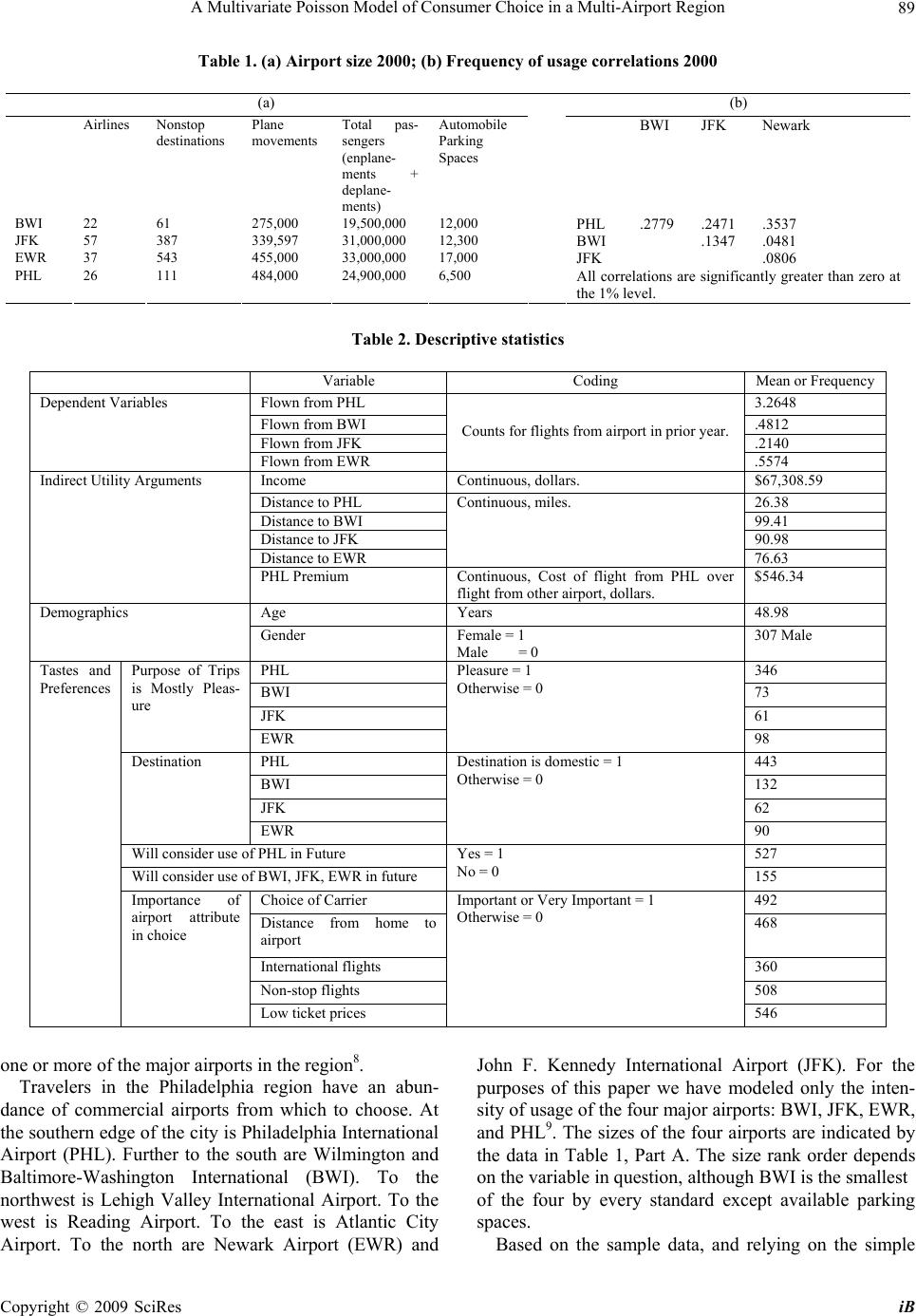

A Multivariate Poisson Model of Consumer Choice in a Multi-Airport Region 89
Table 1. (a) Airport size 2000; (b) Frequency of usage correlations 2000
(a) (b)
Airlines Nonstop
destinations
Plane
movements
Total pas-
sengers
(enplane-
ments +
deplane-
ments)
Automobile
Parking
Spaces
BWI JFK Newark
BWI 22 61 275,000 19,500,000 12,000 PHL .2779 .2471 .3537
JFK 57 387 339,597 31,000,000 12,300 BWI .1347 .0481
EWR 37 543 455,000 33,000,000 17,000 JFK .0806
PHL 26 111 484,000 24,900,000 6,500 All correlations are significantly greater than zero at
the 1% level.
Table 2. Descriptive statistics
Variable Coding Mean or Frequency
Flown from PHL 3.2648
Flown from BWI .4812
Flown from JFK .2140
Dependent Variables
Flown from EWR
Counts for flights from airport in prior year.
.5574
Income Continuous, dollars. $67,308.59
Distance to PHL 26.38
Distance to BWI 99.41
Distance to JFK 90.98
Distance to EWR
Continuous, miles.
76.63
Indirect Utility Arguments
PHL Premium Continuous, Cost of flight from PHL over
flight from other airport, dollars.
$546.34
Age Years 48.98 Demographics
Gender Female = 1
Male = 0
307 Male
PHL 346
BWI 73
JFK 61
Purpose of Trips
is Mostly Pleas-
ure
EWR
Pleasure = 1
Otherwise = 0
98
PHL 443
BWI 132
JFK 62
Destination
EWR
Destination is domestic = 1
Otherwise = 0
90
Will consider use of PHL in Future 527
Will consider use of BWI, JFK, EWR in future
Yes = 1
No = 0 155
Choice of Carrier 492
Distance from home to
airport
468
International flights 360
Non-stop flights 508
Tastes and
Preferences
Importance of
airport attribute
in choice
Low ticket prices
Important or Very Important = 1
Otherwise = 0
546
one or more of the major airports in the region8.
Travelers in the Philadelphia region have an abun-
dance of commercial airports from which to choose. At
the southern edge of the city is Philadelphia International
Airport (PHL). Further to the south are Wilmington and
Baltimore-Washington International (BWI). To the
northwest is Lehigh Valley International Airport. To the
west is Reading Airport. To the east is Atlantic City
Airport. To the north are Newark Airport (EWR) and
John F. Kennedy International Airport (JFK). For the
purposes of this paper we have modeled only the inten-
sity of usage of the four major airports: BWI, JFK, EWR,
and PHL9. The sizes of the four airports are indicated by
the data in Table 1, Part A. The size rank order depends
on the variable in question, although BWI is the smallest
of the four by every standard except available parking
spaces.
Based on the sample data, and relying on the simple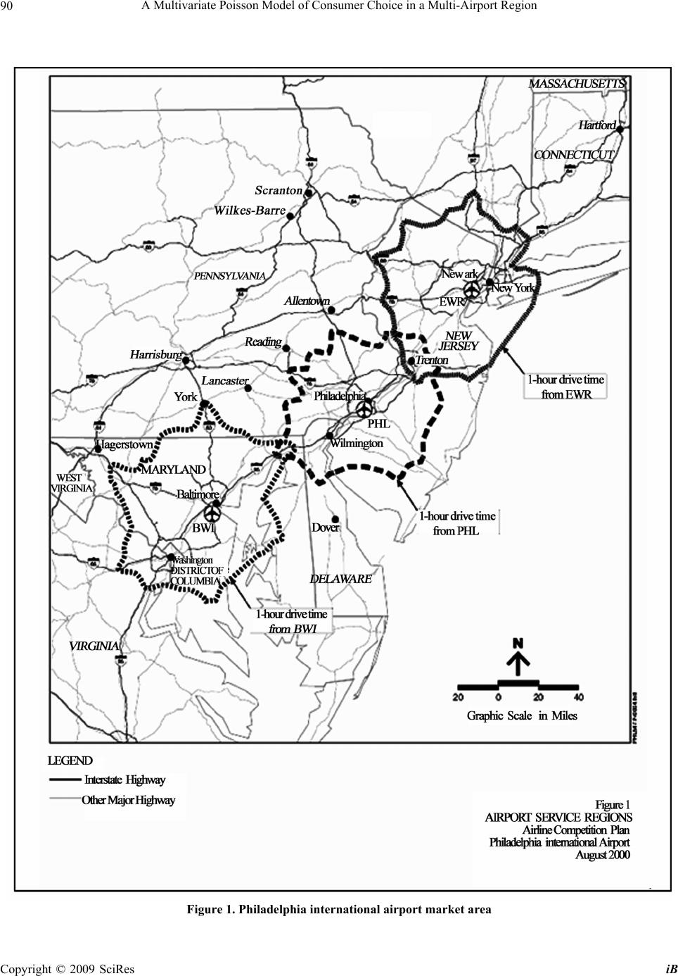

A Multivariate Poisson Model of Consumer Choice in a Multi-Airport Region 90
Figure 1. Philadelphia international airport market area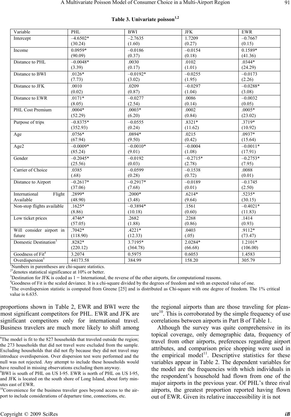

A Multivariate Poisson Model of Consumer Choice in a Multi-Airport Region 91
Table 3. Univariate poisson1,2
Variable PHL BWI JFK EWR
Intercept –4.6502*
(30.24)
–2.7635
(1.60)
1.7209
(0.27)
–0.7667
(0.15)
Income 0.0959*
(90.09)
–0.0186
(0.37)
–0.0154
(0.18)
0.1589*
(41.36)
Distance to PHL –0.0048*
(3.39)
.0030
(0.17)
.0102
(1.01)
.0344*
(24.29)
Distance to BWI .0126*
(7.73)
–0.0192*
(3.02)
–0.0255
(1.95)
–0.0173
(2.26)
Distance to JFK .0010
(0.02)
.0209
(0.87)
–0.0297
(1.04)
–0.0288*
(3.08)
Distance to EWR .0171*
(8.05)
–0.0277
(2.54)
.0086
(0.14)
–0.0032
(0.05)
PHL Cost Premium .0004*
(52.29)
.0003*
(6.20)
.0002
(0.84)
.0005*
(23.02)
Purpose of trips –0.8375*
(352.93)
–0.0555
(0.24)
.8321*
(11.62)
.3719*
(10.92)
Age .0756*
(67.94)
.0894*
(9.50)
.0215
(0.42)
.0937*
(15.64)
Age2 –0.0009*
(85.24)
–0.0010*
(9.01)
–0.0004
(1.08)
–0.0011*
(17.91)
Gender –0.2045*
(25.56)
–0.0192
(0.03)
–0.2715*
(2.78)
–0.2753*
(7.95)
Carrier of Choice .0385
(.68)
–0.0599
(0.28)
–0.1538
(0.72)
.0088
(0.01)
Distance to Airport –0.2617*
(37.06)
–0.2917*
(7.68)
–0.0189
(0.01)
–0.1745
(2.50)
International Flight
Available
.2899*
(48.90)
.2000*
(3.48)
.6214*
(9.64)
.5235*
(30.15)
Non-stop flights available .1625*
(8.86)
–0.3894*
(10.18)
.1561
(0.60)
–0.4021*
(11.83)
Low ticket prices .4746*
(57.05)
.2682
(1.88)
.2268
(0.86)
.1414
(0.93)
Will consider airport in
future
.7042*
(118.90)
.4221*
(12.33)
.0403
(.05)
.9112*
(73.47)
Domestic Destination3 .8282*
(220.12)
3.7195*
(364.78)
2.0284*
(66.68)
1.2101*
(106.00)
Goodness of Fit4 3.2074 0.5975 0.6053 1.4583
Overdispersion5 44173.58 384.99 158.20 305.79
1Numbers in parentheses are chi-square statistics.
2*denotes statistical significance at 10% or better.
3Destination for JFK is coded as 1 = International, the reverse of the other airports, for computational reasons.
4Goodness of Fit is the scaled deviance. It is a chi-square divided by the degrees of freedom and with an expected value of one.
5The overdispersion statistic is computed from Greene [25] and is distributed as Chi-square with one degree of freedom. The 1% critical
value is 6.635.
proportions shown in Table 2, EWR and BWI were the
most significant competitors for PHL. EWR and JFK are
significant competitors only for international travel.
Business travelers are much more likely to shift among
the regional airports than are those traveling for pleas-
ure10. This is corroborated by the simple frequency of use
correlations between airports in Part B of Table 1.
Although the survey was quite comprehensive in its
topical coverage, only demographic data, frequency of
travel from other airports, preferences regarding airport
attributes, and comparison price shopping were used in
the empirical model11. Descriptive statistics for these
variables appear in Table 2. The dependent variables for
the model are the frequencies with which individuals in
the respondent’s household had flown from one of the
8The model is fit to the 827 households that traveled outside the region;
the 273 households that did not travel were excluded from the sample.
Excluding households that did not fly because they did not travel may
introduce overdispersion. Over dispersion test were performed and the
null was not rejected. Any attempt to include these households would
have resulted in missing observations excluding them anyway.
9BWI is south of PHL on US I-95. EWR is north of PHL on US I-95,
and JFK is located on the south shore of Long Island, about forty min-
utes east of EWR.
10Convenience for the business traveler goes beyond access to the air-
p
ort to include considerations of departure time, connections, etc.
major airports in the previous year. Of PHL’s three rival
airports, the greatest proportion reported having flown
out of EWR. Given its relative inaccessibility it is not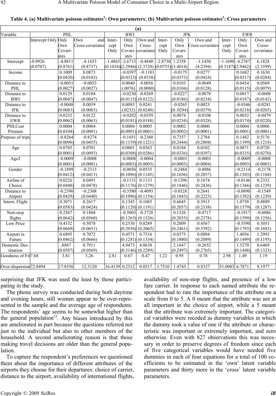

A Multivariate Poisson Model of Consumer Choice in a Multi-Airport Region 92
Table 4. (a) Multivariate poisson estimates1: Own paramet ers ; (b) Multivariate poisson estimates1: Cross parameters
(a)
Variable PHL BWI JFK EWR
Intercept Only Only
Own
Covari-
ates
Own and
Cross-covariates
Inter-
cept
Only
Only
Own
Covari-
ates
Own and
Cross-
covariates
Inter-
cept
Only
Only
Own
Covari-
ates
Own and
Cross-covariates
Inter-
cept
Only
Only
Own
Covari-
ates
Own and
Cross-
covariates
Intercept -0.9926
(0.0707)
–4.8811
(0.8761)
–4.1653
(0.8737)
–1.4863
(0.1034)
–2.6713
(2.2946)
–0.4840
(2.3720)
–2.8730
(0.0755)
1.2358
(3.4014)
–1.1430
(4.2394)
–1.1690
(0.3187)
–4.2767
(2.9462)
6.1828
(2.3599)
Income 0.1009
(0.0420)
0.0873
(0.0103)
–0.0397
(0.0323)
–0.1101
(0.0338)
–0.0175
(0.0373)
0.0277
(0.0424)
0.1682
(0.0317)
0.1630
(0.0284)
Distance to
PHL
–0.0051
(0.0027)
–0.0053
(0.0027)
0.0040
(.0076)
0.0056
(0.0080)
0.0103
(0.0104)
–0.0049
(0.0128)
0.0454
(0.0115)
0.0569
(0.0079)
Distance to
BWI
0.0129
(0.0047)
0.0104
(0.0047)
–0.0230
(0.0115)
–0.0269
(0.0122)
–0.0227
(0.0186)
–0.0078
(0.0234)
0.0017
(0.0187)
–0.0608
(0.0142)
Distance to
JFK
–0.0048
(0.0083)
0.0039
(0.0083)
0.0083
(.0232)
0.0241
(0.0240)
–0.0265
(0..0294)
0.0023
(0.0379)
–0.0346
(0.0218)
–0.0281
(0.0203)
Distance to
EWR
0.0232
(0.0062)
0.0122
(0.0063)
–0.0202
(0.0181)
–0.0359
(0.0188)
0.0074
(0.0234)
–0.0108
(0.0328)
0.0032
(0.0174)
–0.0479
(0.0220)
PHLCost
Prmium
0.0004
(0.0104)
0.0004
(0.0001)
0.0004
(0.0001)
0.0005
(0.0001)
0.0002
(0.0002)
0.0000
(0.0001)
0.0004
(0.0001)
0.0006
(0.0001)
Purpose of trips –0.8264
(0.0096)
–0.8274
(0.0455)
–0.1651
(0.1159)
–0.2360
(0.1221)
0.7357
(0.2444)
3.2784
(0.2804)
0.1482
(0.1399)
0.5176
(0.1218)
Age 0.0785
(0.0001)
0.0701
(0.0093)
0.0801
(0.0308)
0.0363
(0.0286)
0.0184
(0.0336)
0.0102
(0.0397)
0.0871
(0.0335)
0.0720
(0.0270)
Age2 –0.0009
(0.0001)
–0.0008
(0.0001)
–0.0008
(0.0003)
–0.0004
(0.0003)
–0.0003
(0.0003)
–0.0003
(0.0004)
–0.0009
(0.0003)
–0.0008
(0.0003)
Gender –0.1899
(0.0412)
–0.2313
(0.0413)
–0.0056
(0.1096)
0.0535
(0.1145)
–0.2484
(0.1656)
–0.4986
(0.2057)
–0.2114
(0.1303)
–0.2178
(0.1104)
Airline of
Choice
0.0226
(0.0448)
0.0491
(0.0478)
–0.1131
(0.1176)
0.1133
(0.1279)
–0.1296
(0.1846)
0.1674
(0.2436)
–0.0146
(0.1366)
0.2332
(0.1239)
Distance to
Airport
–0.2390
(0.0429)
–0.2308
(0.0440)
–0.3580
(0.1096)
–0.4093
(0.1154)
–0.0528
(0.1843)
0.2641
(0.2223)
–0.0890
(0.1582)
–0.1549
(0.1239)
Intern. Flight 0.3071
(0.0583)
0.2617
(0.0424)
0.1345
(0.1120)
0.1085
(0.1191)
0.6645
(0.2057)
0.5913
(0.2338)
1.0758
(0.1579)
0.4809
(0.1287)
Non-stop
flights
0.2567
(0.0642)
0.1804
(0.0560)
–0.5003
(0.1265)
–0.3728
(0.1326)
0.1326
(0.2035)
–0.4717
(0.2378)
–0.1917
(0.1599)
–0.6086
(0.1256)
Low Price 0.4132
(0.0669)
0.5078
(0.0651)
0.2530
(0.2036)
0.0289
(0.2065)
0.2009
(0.2461)
0.4567
(0.3392)
–0.5590
(0.1793)
0.3051
(0.1683)
Airport in
Future
0.6895
(0.0462)
0.7072
(0.0666)
0.4571
(0.1281)
0.7316
(0.1334)
0.0375
(0.1880)
0.0884
(0.2089)
1.4036
(0.1499)
1.2993
(0.1195)
Domestic Des-
tination
.8867
(0.0587)
0.7911
(0.0569)
4.9473
(0.3146)
4.0638
(0.2289)
2.1647
(0.2497)
–0.2652
(0.2765)
1.5270
(0.1448)
0.6469
(0.1323)
Goodness of Fit 7.68 3.813.26 2.810.670.47 1.220.950.78 2.98 1.49 1.19
Over-dispersion72.8494 17.835612.3120 16.41390.25120.05171.75101.47430.8327 51.0083 6.78718.1977
surprising that JFK was used the least by those partici-
pating in the study.
The phone survey was conducted during both daytime
and evening hours, still women appear to be over-repre-
sented in the sample and the average age of respondents.
The respondents’ age seems to be somewhat higher than
the general population12. Any biases introduced by this
are ameliorated in part because the questions referred not
just to the individual but also to other members of the
household. A second ameliorating reason is that those
making travel decisions are older than the general popu-
lation.
To capture the respondent’s preferences we questioned
them about the importance of different attributes of the
airports they choose for their departures: choice of carrier,
distance to the airport, availability of international flights,
availability of non-stop flights, and presence of a low
fare carrier. In response to each named attribute the re-
spondent had to rate the importance of the attribute on a
scale from 0 to 5. A 0 meant that the attribute was not at
all important in the choice of airport, while a 5 meant
that the attribute was extremely important. The categori-
cal variables were recoded as dummy variables in which
the dummy took a value of one if the attribute or charac-
teristic was important or extremely important, and zero
otherwise. Even with 827 observations this was neces-
sary in order to preserve degrees of freedom since each
of five categorical variables would have needed five
dummies in each of four equations for a total of 100 co-
efficients to be estimated in the ‘own’ latent variable
parameters and thirty more in the ‘cross’ latent variable
parameters.

A Multivariate Poisson Model of Consumer Choice in a Multi-Airport Region 93
(b)
β12
PHL-BWI
β13
PHL-JFK
β14
PHL-EWR
β23
BWI-JFK
β24
BWI-EWR
β34
JFK-EWR
Intercept Only
Constant –1.4203
(0.8889)
–2.1834
(0.1913)
–1.5498
(0.0200)
–6.4847
(0.0728)
–4.4334
(0.1463)
–3.4124
(0.0624)
Own Covariates Only
Constant –3.3126
(0.1819)
–11.1798
(8.2713)
–1.6524
(0.0794)
–5.6071
(10.3666)
–11.9811
(0.5727)
–4.8901
(0.4009)
Own- and Cross-covariates
Constant –158.9580
(70.0804)
–186.1933
(65.0043)
–35.7531
(11.0068)
–168.7721
(57.3307)
–98.3382
(116.3201)
–48.4551
(20.3832)
Gender 0.6821
(3.2583)
9.0643
(3.7696)
–0.1828
(0.4854)
–12.1547
(4.6281)
–5.7411
(8.1581)
3.3350
(2.2894)
Income 2.4149
(0.9592)
0.7534
(1.1107)
0.5740
(0.1370)
3.2353
(0.9174)
–1.6019
(1.8122)
–1.1716
(0.5320)
Age 3.4240
(2.1153)
4.3864
(1.7690)
0.4212
(0.1264)
2.5693
(1.7027)
–0.4105
(3.6229)
1.7731
(0.7870)
Age2 –0.0342
(0.0210)
–0.0291
(0.0143)
–0.0038
(0.0012)
–0.0339
(0.0177)
0.0066
(0.0427)
–0.0296
(0.0115)
Carrier 17.2770
(9.7328)
–0.5263
(2.6063)
–0.3163
(0.4169)
–5.8861
(11.2654)
–30.2447
(5.4843)
2.5751
(1.9926)
Distance 7.5194
(4.7410)
–5.3075
(2.3233)
–1.3789
(0.4175)
6.8751
(3.5287)
9.8577
(11.0292)
1.1548
(2.1540)
Interna-
tional
0.1996
(2.9954)
–9.0871
(3.8296)
0.3889
(0.4060)
3.9001
(4.0220)
11.9829
(3.1542)
3.8812
(3.3086)
Non-stop –10.8234
(5.9471)
10.4281
(5.2275)
2.4725
(0.7993)
4.3507
(7.0232)
–1.6884
(8.1904)
4.0210
(2.9817)
Pricing 5.6050
(3.7408)
–10.6328
(5.6392)
–3.3539
(0.9096)
–9.417
(12.9732)
12.5169
(8.0006)
3.7280
(3.6626)
Will Use
PHL
7.6172
(4.4773)
–4.2938
(5.9367)
–4.3224
(0.9744)
-- -- --
Will Use
Other
–16.3339
(6.7274)
–13.4868
(7.9894)
–6.5853
(1.3802)
–8.8263
(5.4286)
–10.7623
(4.7005)
–5.1143
(3.7945)
PHL Pre-
mium
–0.0067
(0.0046)
0.0004
(0.0049)
0.0020
(0.0006)
-- -- --
Distance to
i
–0.2101
(0.3202)
0.3084
(0.1157)
–0.0014
(0.0160)
0.2039
(0.2592)
0.1501
(0.3319)
0.0499
(0.1969)
Destination
from i
16.2027
(10.2507)
–1.6024
(3.6469)
–0.7071
(0.9399)
7.1347
(15.5945)
35.4171
(4.6455)
15.7171
(4.9331)
Distance to
j
0.0583
(0.1192)
–0.2442
(0.1237)
0.1003
(0.0222)
0.7135
(0.1322)
0.71345
(0.3797)
–0.0265
(0.1809)
Destination
from j
8.5510
(4.0695)
44.2165
(14.4379)
17.2567
(9.7092)
20.4702
(6.4014)
–14.7535
(8.6005)
6.5796
(2.8247)
Purpose i –9.4457
(5.2732)
13.7023
(4.9055)
3.2956
(0.9270)
2.7957
(5.0255)
–3.0041
(6.8273)
–11.0594
(4.3178)
Purpose j 5.5829
(2.3648)
–24.4502
(9.4837)
–1.8782
(0.6858)
–11.7110
(6.6219)
14.3912
(6.0686)
–1.4067
(2.4231)
1Numbers in parentheses are standard errors.
Only the presence of international flights was of little
or no importance to PHL users. This is somewhat sur-
prising given PHL’s notoriously poor international ser-
vice at that time. A surprising 20% of respondents re-
ported that they had compared a fare out of PHL with
fares available at other airports. As a follow-up they were
also asked about the fare difference in that comparison.
For the 165 travelers that made the comparison the aver-
age fare premium was $546.34.13
4. Empirical Results
The index function that is used here is a mix of indirect
utility arguments, such as price premium for flying from
PHL, actual distance to the airport and income14, and
tastes and preferences, such as the assessment that using
the carrier of choice is important. The survey results in-
cluded data on the respondents’ age and gender15.
The signs on age and gender are indeterminate a priori,
although it is reasonable to expect that frequency of fly-
ing and age is a nonlinear relationship. The marginal
effect of an increase in income on the probability of us-
ing a more distant airport could be negative or positive.
As an individual’s income rises she finds the opportunity
cost of increased travel time to a more distant airport to
be a disincentive to using that airport16. On the other
hand service and fare might overcome that (dis)incentive.

A Multivariate Poisson Model of Consumer Choice in a Multi-Airport Region 94
Table 5. Marginal effects on mean number of trips
Univariate Multivariate
PHL BWI JFK EWR PHL BWI JFK EWR
DPHL –0.012 0.0003 0.0011 0.0095 –0.0155 0.0002 –0.0002 0.0114
DBWI 0.0314 –0.0018 –0.0027 –0.0048 0.0303 –0.0010 –0.0003 –0.0122
DJFK 0.0025 0.0020 –0.0032 –0.0079 0.0114 0.0009 0.0001 –0.0056
DEWR 0.0426 –0.0027 0.0009 –0.0009 0.0356 –0.0013 –0.0004 –0.0010
Income 0.2388 –0.0073 –0.0016 0.0438 0.2545 –0.0039 0.0001 0.0328
Cost Premium 0.0010 0.0001 0.00002 0.0001 0.0012 0.00002 0.0000 .0001
Age –0.0313 –0.0033 –0.0019 –0.0039 –0.0241 –0.0001 –0.0007 –0.0013
Carrier 0.0955 –0.0058 –0.0167 0.0002 0.9183 0.0041 0.0062 0.0460
International 0.7382 0.0196 0.0705 0.1510 0.5652 0.0039 0.0236 0.1007
Non-stop 0.3979 –0.0396 0.0165 –0.1166 0.3749 –0.0142 –0.0190 –0.1329
Low cost 1.1057 0.0249 0.0235 0.0381 1.0019 0.0010 0.0162 0.0586
Distance –0.6642 –0.0294 –0.0021 –0.0487 –0.0674 –0.0287 –0.0127 –0.0311
Purpose –2.0045 –0.0052 0.1310 0.1188 –2.3191 –0.0146 0.9475 –0.0000
Domestic 2.0526 2.1500 0.6083 0.5686 1.2798 2.0302 0.286 1.7834
Will Use 1.622 0.0469 0.0494 0.3455 1.9068 0.0638 .0043 0.4159
Gender –0.5239 –0.0018 –0.0397 –0.1039 –0.6965 0.0036 –0.0079 –0.0447
The indirect utility arguments include whether the re-
spondent had obtained the price of a comparable flight
from an airport other than Philadelphia and what the
price difference turned out to be. One would expect that a
consumer’s price research would induce them to use the
flight departing from the cheaper airport.
Tastes and preferences are modeled from a sequence
of questions regarding factors that the traveler finds im-
portant in choice of airport as well as the purpose and
destinations of trips taken. The survey17 asked for an
ordered response to eight questions regarding airport
attributes, although only five are used here18. Survey
participants could rank an attribute of an airport and its
services from 0 to 5; a response of 0 indicated that the
factor was not at all important, a response of 5 indicated
that the factor was extremely important in the decision
making process. Table 2 provides the variables and cor-
responding descriptive statistics.
If ability to choose a particular airline or fly an inter-
national carrier is important then one would expect that
the respondent would be more likely to have flown out of
JFK, all other things equal, given its much wider choice
of carriers (See Table 1). People for whom distance to
the airport is an important consideration would be less
likely to have flown out of JFK. If finding a nonstop
flight is extremely important then the respondent should
be more likely to have flown out of EWR. The folk wis-
dom at the time of the survey was that because USAir
had dominated PHL for so long it had the ability to
charge higher fares. There was no similar carrier domi-
nance in the other three airports. Therefore, if price is an
extremely important consideration then a respondent
should be less likely to have flown out of PHL in the
preceding year.
Both univariate, Table 3, and multivariate, Table 4,
Poisson models were fit to the data19. For both sets of
results measures of goodness of fit and over dispersion
are included. Three specifications of the multivariate
model for each airport are reported in Table 4. The first
specification assumed homogeneity across all respon-
dents and involved estimating the 10x1 vector θ of Equa-
tion (5) as though all coefficients except the intercept on
the covariates of Equation (7) were zero. The second
specification assumed heterogeneity in the θi (i=1, 2, 3, 4)
but homogeneity in the covariance terms, θij (i,j = 1,2,3,4
and i<j). In the third specification all of the θ were
treated as heterogeneous across the respondents.
11Household size was included in the survey, but was not significant in
any of the model specifications. If the dependent variable had been the
number of tickets purchased for flights from each airport then house-
hold size would have been essential. If the trip or journey is the de-
p
endent variable then the number of individuals making the trip is
irrelevant. If, say BWI, is the cheaper and closer airport for one mem-
b
er of the family then it is still cheaper and closer when they travel as a
group.]
12Only respondents indicating that they were over 18 were included in
the survey. The survey was conducted only among landline telephone
subscribers. In 2004 the percent of the population with ‘cell phone
only’ service was 6.3 percent in metropolitan areas [26].
13Or $109 when averaged over the entire sample.
14At the time of the phone survey the respondent’s 3 digit telephone
exchange was captured. Using the airport phone exchanges it was then
p
ossible to retrieve the distance from the respondent to each of the
airports from a commercially available database [27]. The same data-
base was used to code income as the median for residents of the par-
ticular telephone exchange. As part of the survey participants were
asked to respond categorically to a question about their household
income. Of course not all respondents answered that question. The
correlation between our income construct and the categorical responses
was 0.87.
In comparing the univariate and multivariate results
there is essentially no change in the sign pattern on the
covariate coefficients or which coefficients are signifi-
cant20. The goodness of fit statistics21 are roughly com-
parable for the two models. The biggest difference arises
in the over dispersion statistics22. For the unvaried model
the null hypothesis of no over dispersion is rejected for

A Multivariate Poisson Model of Consumer Choice in a Multi-Airport Region95
each of the four airports23. With the exception of the in-
tercepts only specification for PHL the null of no over
dispersion is never rejected for the multivariate model. It
would appear that the latent variable specification allow-
ing for covariance between airport usage eliminates the
over dispersion problem apparent in the univariate mod-
els. To put it somewhat differently, the univariate model
is not correctly specified. Finally, the θij terms, the count
covariance latent variables, are statistically different from
zero in nine out of twelve instances in the intercepts only
and own covariates only versions of the multivariate
Poisson models.
Since particular covariates appear in both the coeffi-
cient vector of the own-latent variables and the cross-
latent variables it is more useful to consider the incre-
mental effects of the covariates on the mean response.
The results for both the univariate and multivariate mod-
els are summarized in Table 5: Marginal effects on mean
number of trips24. In the case of continuous covariates the
marginal effects are derivatives. In the case of the dis-
crete covariates the model is evaluated for the two values
of the dummy variable and the difference computed. All
derivatives and differences are evaluated at the means of
the covariates.
The effect of distance from a given airport on the fre-
quency of choice of that airport has the expected negative
sign for PHL, BWI and EWR. The sign for JFK is posi-
tive due to the dominant cross effect between JFK and
BWI in part B or Table 4; as one gets further from either
one of them one uses one or the other more often. A
greater distance from any of the other three airports will
increase the frequency of flights from PHL. As a re-
spondent gets further from PHL or JFK, her mean usage
of BWI increases. However, as they become more distant
from EWR their mean usage of BWI decreases. This is
attributable to the geography of the region and cross ef-
fects. If one is on the north side of PHL and moves fur-
ther from EWR then one must be getting closer to PHL,
hence there is a shift from BWI to PHL. If one is to the
south of PHL and one gets further from EWR then one
must be getting closer to BWI and further from PHL. It
may be that the attributes other than distance overwhelm
the distance effect for BWI. Mean usage of JFK is de-
creasing in distance from any of the other three airports.
This is easy to understand for EWR since a greater dis-
tance from EWR means that one is more distant from
JFK. If one is more distant from BWI than one must be
closer to JFK, but the total distance remains great and
PHL is relatively more attractive as a choice. The relative
attraction of PHL overwhelms any gain that might be
attributed to being further away from PHL, hence the
negative sign. The negative sign on distance from JFK in
the EWR mean is explained by the fact that being further
from JFK means being further from EWR and closer to
PHL. Similarly, being further from BWI moves one
closer to EWR, but the proximity effect of PHL is over-
whelming.
Higher income results in an increase in the mean use
of PHL, JFK and EWR, although the effect on use of
JFK is numerically very much smaller than that for either
PHL or EWR. The sign on income is negative for BWI.
As it happens, mean income increases with distance from
BWI so there is a confounding income-distance effect for
the use of BWI.
15Gender of respondent may be serving as a proxy for many different
aspects of the airport choice process. Including it in the models has a
small effect on statistical efficiency, but excluding a relevant variable
introduces bias.
16The geographically more distant airport does not always mean greater
travel time. Traffic congestion, high speed rail links, etc. may result in
less travel time to the more distant airport. For the airports in the region
under study greater distance translates to greater travel time.
17The survey instrument is available from the authors.
18The omitted questions include ease of parking, ease of check-in, and
p
resence of public transit. For any given airport the variability in cate-
gorical rating was quite narrow so the varia
b
les were omitted from the
analysis.
19The univariate model was fit using PROC GENMOD in SAS. The
multivariate EM estimation algorithm was programmed in MATLAB.
The starting values for the MATLAB program were taken from the
univariate results. The convergence criterion for the EM algorithm was
a percent change in the empirical log likelihood of less than 1x10-12.
20Similar sign pattern, statistical significance and coefficient magnitude
should not be confused with goodness of fit. The goodness of fit statis-
tics are higher in the multivariate specification. Even if the covariates
of the covariance structure were not significant for a specific sample in
the multivariate model it would not reduce the importance of the ap-
p
roach.
21The goodness of fit statistic is the scaled deviance (SAS 9.0).
22The over dispersion statistic is the lagrange multiplier statistic from
Greene [25].
23It is worth noting that the over dispersion in the univariate models
leads to overstating the significance of the individual coefficients.
At the time of the survey the folk wisdom was that as a
consequence of USAir’s dominance of PHL that fares
out of PHL were higher than the other airports and that
travelers would use the other airports to get lower fares.
In Table 5 the effect of a greater PHL premium is to in-
crease usage of the other airports. Unfortunately, there is
also a positive effect on the mean usage of PHL. This
may be due in part to the fact that the effects of distance
overwhelm any cost advantage to flying from another
airport [28]. This could be thought of as a barrier to cus-
tomer mobility that results in limit pricing by the carrier:
US Airways might charge a premium with the expecta-
tion that customers will not defect to another airport.
The coefficients on covariates age and its square are
respectively positive and negative, although their aggre-
gate effect on mean use is negative for all four airports.
The gender effect is that women fly less often than men
from all airports but BWI. If the purpose of one’s trips
was mostly for pleasure then one would use JFK more
frequently and the others less frequently, on average. At
the time of the survey PHL’s choice of carrier, interna-
tional, and non-stop service was poor. When traveling for

A Multivariate Poisson Model of Consumer Choice in a Multi-Airport Region 96
pleasure, and time in transit has a lower opportunity cost,
one might be more inclined to use a more inconvenient
airport in order to get the desired service attributes. If
destination of the trips was domestic then one was more
likely to use PHL, BWI and EWR. Since domestic desti-
nation for JFK was coded as the reverse of the other three
airports the sign must be switched25. Thus, if the destina-
tion of the trips was international then travelers increased
their mean use of JFK.
Six taste and preference questions were included in
the specifications: Importance of choice of carrier, im-
portance of international flights, importance of avail-
ability of non-stop flights, importance of low fare carri-
ers, importance of distance to the airport, and willing-
ness to use the airport again26. In magnitude, the mar-
ginal effect of international flight availability on mean
usage of PHL is much greater than that for the other
airports due to the size of the cross covariates in part B
of Table 5; at the time of the survey PHL had the repu-
tation of being very inconvenient for international trav-
elers. Apparently, if an international flight is available
at all three airports then a consumer in the PHL market
area will be more likely to travel from PHL. Apparently
the management at PHL had at least a visceral under-
standing of this. Since the time of the survey PHL has
constructed a new international terminal in order to ad-
dress the needs of overseas travelers in its market.
When the availability of non stop flights is an important
consideration travelers use PHL more often and are less
likely to use the other airports as often. Table 1 shows
that two airports had better non-stop service than PHL,
and at that time PHL was not a hub for any of its carri-
ers27. The importance of the presence of a low cost car-
rier also had its greatest impact on PHL. Again, this is
not surprising since at the time of the survey Airtran, a
low cost carrier, had only recently come to PHL. Since
the time of the survey PHL has built a short commuter
runway, built another domestic service terminal, and
added a second low cost carrier28. When distance to the
airport is an important consideration the effect for all
four airports is to reduce the mean number of trips,
consistent with the findings for actual distance. Finally,
a willingness to use the given airport again will increase
the mean use of any of the airports.
5. Conclusions
A multivariate Poisson specification was used to analyze
data on the choice of airport from a phone survey of the
Philadelphia International Airport (PHL) market. The
survey polled nearly 5000 homes to generate a usable
sample of 827 respondents that had traveled outside the
region29. In airport choice studies the respondents are
intercepted in an airport and queried about the choice that
has brought them to that location instead of others in the
choice set. The corresponding appropriate analytical
methodology is multinomial logit or probit. The phone
survey used here asked respondents to report on all of
their air travel in the prior year. Hence, for each respon-
dent there was a count of the number of times she had
flown from each of the four airports in the region. Since
the count data represents the results of choices made re-
peatedly over many short time periods it is in principle
Poisson distributed.
Since each respondent was flying from among four
major airports the correct specification is multivariate
Poisson. The multivariate Poisson, which does not have a
closed form, can be recast as a latent variables problem
that results in marginal distributions for correlated Pois-
son variates. The parameters in the multivariate Poisson
model were estimated using an expectation maximization
algorithm.
24There are no significance tests indicated in Table 5 since they are
unnecessary. One or more of the coefficients on each variable for a
given airport is significant so the corresponding effect on the rate
p
arameter will also be significant. The Poisson rate parameter is
recovered from the tabled numbers by Equation (7). The mapping
from the estimated coefficients to the rate parameter is an affine
transformation. Affine transformations preserve ordering and dis-
tance. Also, the usual test statistics are scale invariant. Hence, if a
significant relationship exists before the transformation it will be
significant after the transformation. Greene [25] addresses the same
sort of question.
25Among those in the sample who had flown from JFK the proportion
using that airport to get international service was much greater than
those using the airport for domestic service, the reverse of the other
airports. As it happened, this switch also resulted in the EM algorithm
converging more rapidly.
26Willingness to use the airport again is a taste and preference variable
to the extent that it reflects changing proclivity on the basis of prio
r
experience. The neoclassical model assumes stable preferences, but in
reality preferences do change in the aftermath of experience.
27Although USAir dominated the airport by any measure, PHL was not
its east coast hub. Its hub remained in Pittsburgh even though it had
more traffic in and out of PHL.
28Southwest Airlines. The addition of new terminals, another discount
carrier and more international service has resulted in PHL being the
second fastest growing airport in the world, behind only Beijing.
29A response rate of 22% is typical for a phone survey that employs no
special devices to increase response rates and rates of cooperation [29].
An airport’s own-distance had the expected negative
impact on mean usage of the airport, although the cross
effects were somewhat mixed. Mean usage was found to
be increasing in income for PHL, but was decreasing for
the other airports, reflecting the increasing value of re-
spondents’ time as their income rises. On balance the
quadratic form in respondent’s age resulted in less fre-
quent flights among older respondents. A rising fare
premium for using PHL resulted in higher mean use for
Newark (EWR), Baltimore (BWI) and New York (JFK).
The fare premium was also positive for use of PHL, re-
flecting that market power of PHL’s dominant carrier at
the time of the survey. If the destination of flights is do-
mestic (international) then the result is to increase usage
of PHL, BWI and EWR (JFK). Except for JFK, if the

A Multivariate Poisson Model of Consumer Choice in a Multi-Airport Region97
purpose of travel is mostly pleasure then it results in
more travel from JFK and less from the other three air-
ports. The availability of a low cost carrier would result
in more frequent travel.
Since the time of the survey the entry of a new low
cost carrier and the construction of a new international
arrivals terminal have caused PHL usage to increase
dramatically. It experienced a 10.5 percent increase in
passengers in 2005 alone and a 28 percent increase since
2003. In terms of aircraft activity PHL is now the ninth
largest in the world [30].
In summary, given the results of the model, it appears
that at the time of the study airlines at Philadelphia In-
ternational Airport made a profit maximizing decision to
take advantage of their regional monopoly. Their prices
were high enough to extract monopoly rent while losing
only small numbers of passengers to lower cost carriers
at other airports. Hence outmigration of potential pas-
sengers is not a significant constraint on monopoly pow-
er at airports. These results also tend to support smaller
geographic market definitions and perhaps even the prac-
tice of price discrimination. The entry of Southwest into
Philadelphia International Airport may have reclaimed
some marginal travelers that had been going to the com-
peting airports, but the biggest impact will be on fare
competition among airlines already serving PHL.
REFERENCES
[1] Hess, Stephane, and Polak, J., “Mixed logit modeling of
airport choice in multi-airport regions,” Journal of Air
Transport Management, Vol. 11, No. 2, pp. 59–68, 2005.
[2] Hess, Stephane, and Polak, J., “Airport, airline and ac-
cess-mode choice in the san francisco bay area airports,”
Papers in Regional Science, Forthcoming, 2006.
[3] Blackstone, E., Buck, A. J., and Hakim, S., “Determi-
nants of airport choice in a multi-airport region,” Atlantic
Economic Journal, Vol. 34, No. 3, pp. 3–326, September
2006.
[4] Karlis, D., and Meligkotsidou, L., “Multivariate poisson
regression with covariance structure,” Statistics and
Computing, Vol. 15, pp. 255–265, 2005.
[5] Ashford, N. and Benchemam, M., “Passengers’ choice of
airport: An application of the multinomial logit model,”
Transportation Research Record 1147, National Research
Council, Washington, D.C., 1987.
[6] Caves, R. E., Ndoh, N. N., and Pitfield, D. E., “Route
choice modeling applied to the choice between mature
airports and emergent airports in their shadow,” Paper
presented at the 31st RSA European Congress, Lisbon,
Portugal, August 27–30, 1991.
[7] Thompson, A. and Caves, R. E., “The projected market
share for a new small airport in the North of England,”
Regional Studies, Vol. 27, No. 2, pp. 137–147, 1993.
[8] Harvey, G., “Airport choice in a multiple airport region,”
Transportation Research, Vol. 21A, No. 6, pp. 439–449, 1987.
[9] Basar, G. and Bhat, C., “A parameterized consideration set
model for airport choice: An application to the san francisco
bay area,” Transportation Research Part B: Methodological,
Vol. 38, No. 10, pp. 9–904, December 2004.
[10] Hess, S., “An analysis of airport-choice behavior using
the mixed multinomial logit model,” Center for Transport
Studies, Imperial College, London, 2004,
http://www.ersa.org/ersaconfs/ersa04/PDF/61.pdf.
[11] Ishii, J., Jun, S., and VanDender, K., “Air travel choices
in multi-airport markets,” 2005.
[12] Pels, E., Nijkamp, P., and Rietveld, P., “Access to and
competition between airports: A case study for the san
francisco bay area,” Transportation Research Part A: Pol-
icy and Practice, Vol. 37, No. 1, pp. 71–83, January 2003.
[13] Windle, R. and Dresner, M., “Airport choice in a
multi-airport region,” Journal of Transportation Engineer-
ing, Vol. 121, No. 4, pp. 332–338, July–August, 1995.
[14] Gardiner, J., Humphreys, I., and Ison, S., “Freighter
operators’ choice of airport: A three-stage process,”
Transport Reviews, Vol. 25, No. 1, pp. 85–102, January
2005.
[15] Gosling, G. D., “Southern California association of gov-
ernments regional airport demand model: Literature re-
view,” Project #5437, June 2003.
[16] Belden, T. and Ginsberg, T., “A sign of US Airways’
health,” Philadelphia Inquirer, pp. A1 and A4, November
16, 2006.
[17] Morrison, S. A., “Airline service,” in L. L. Deutsch, In-
dustry Studies, 3rd Edition, M. E. Sharpe, Armonk, NY,
pp. 151–152, 2002.
[18] McFadden, D., “Econometric analysis of qualitative re-
sponse models,” In Z. Griliches and M. Intriligator, eds.,
Handbook of Econometrics, North Holland, Amsterdam,
Vol. 2, 1984.
[19] Maddala, G. and Flores-Lagunes, A., “Qualitative re-
sponse models,” in B. Baltagi, ed., A Companion to
Theoretical Econometrics, Blackwell, Oxford, 2001.
[20] Ross, S. M., “Introduction to probability models,” Aca-
demic Press, New York, pp. 174–175, 1980.
[21] Aitchison, J. and Ho, C. H., “The multivariate poisson-
log normal distribution,” Biometrika, Vol. 76, No. 4, pp.
643–653, 1989.
[22] Terza, J. V. and Wilson, P. W., “Analyzing frequencies of
several types of events: A mixed multinomial poisson ap-
proach,” The Review of Economics and Statistics, Vol.
72, No. 1, 108–115, 1990.
[23] Shonkwiler, J. S. and Englin, J., “Welfare losses due to
livestock grazing on public lands: A count data system-
wide treatment,” American Journal of Agricultural Eco-
nomics, Vol. 87, No. 2, pp. 302–313, 2005.
[24] Ben-Akiva, M. and Lerman, S. R., Discrete Choice
Analysis: Theory and Application to Travel Demand, pp.
235–239, the MIT Press, Cambridge, MA, 1985.
[25] Greene, W., Econometric Analysis, 5th Edition, Prentice

A Multivariate Poisson Model of Consumer Choice in a Multi-Airport Region 98
Hall, New York, pp. 743–744, 2003.
[26] Blumberg, S. J., Luke, J. V., and Cynamon, M. L.,
“Telephone coverage and health survey estimates: evalu-
ating the need for concern about wireless substitution,”
American Journal of Public Health, Vol. 96, No. 5, pp.
926–931, May 2006.
[27] Jay Computer Services, 9594 208th Street West, Lakeville,
MN 55044, http://nt.jcsm.com or whttp://www.jcsm.com,
last accessed on 11/09/2006.
[28] Shapiro, H., “The frugal flier: Getting the best buy on an
airline ticket means considering much more than the
fare,” Philadelphia Inquirer, pp. N06, March 28, 2004.
[29] deLeeuw, E. and Hox, J. J., “I am not selling anything: 29
experiments in telephone introductions,” International
Journal of Public Opinion Research, Vol. 16, No. 4, pp.
464–473, 2004.
[30] PHL (Philadelphia International Airport), “2005 numbers
show Philadelphia international airport is now the 9th
busiest airport for aircraft operations,” 2006,
http://www.phl.org/news060228.html.