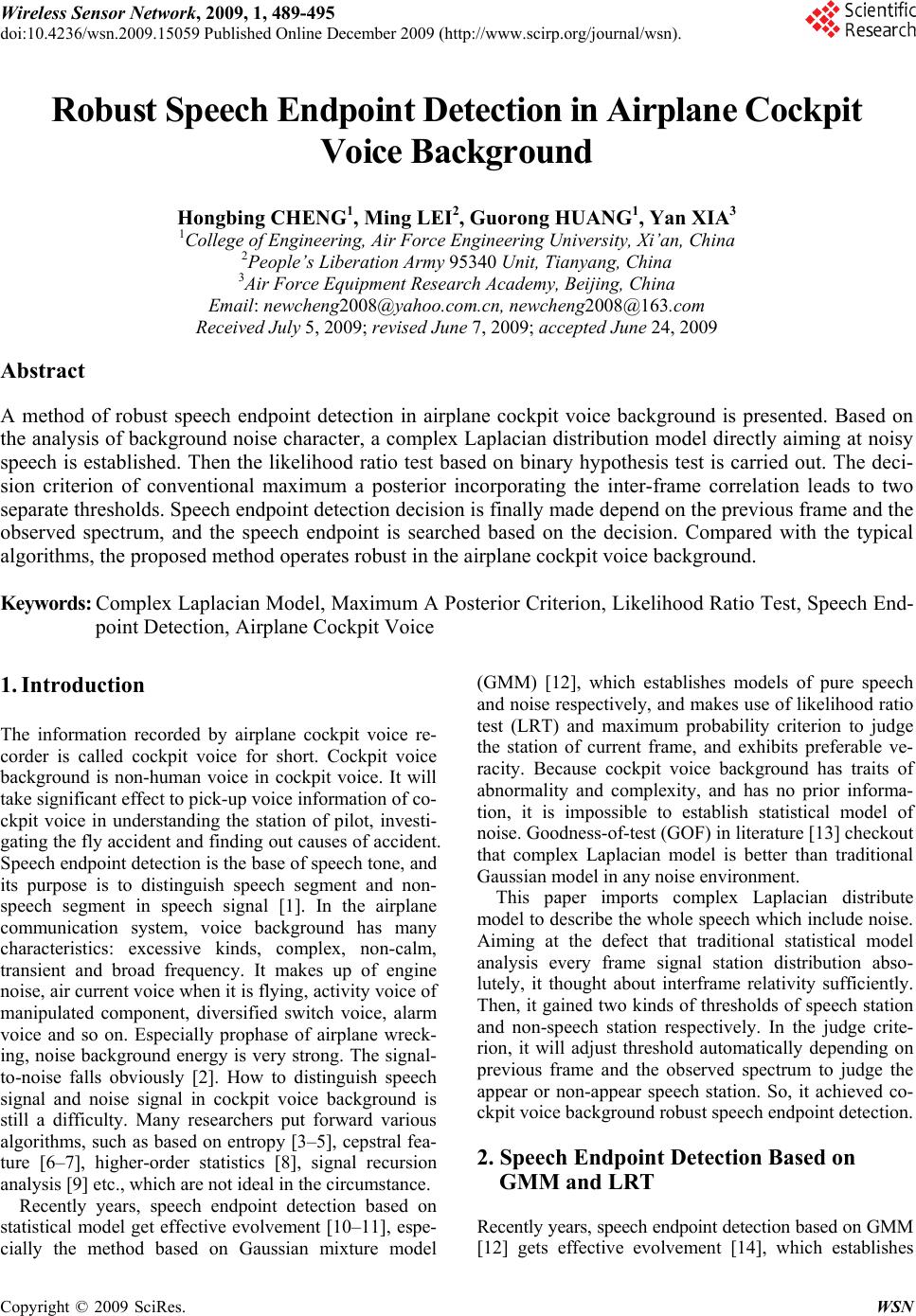Wireless Sensor Network, 2009, 1, 489-495
doi:10.4236/wsn.2009.15059 Published Online December 2009 (http://www.scirp.org/journal/wsn).
Robust Speech Endpoint Detection in Airplane Cockpit
Voice Background
Hongbing CHENG1, Ming LEI2, Guorong HUANG1, Yan XIA3
1College of Engineering, Air Force Engineering University, Xi’an, China
2People’s Liberation Army 95340 Unit, Tianyang, China
3Air Force Equipment Research Academy, Beijing, China
Received July 5, 2009; revised June 7, 2009; accepted June 24, 2009
Abstract
A method of robust speech endpoint detection in airplane cockpit voice background is presented. Based on
the analysis of background noise character, a complex Laplacian distribution model directly aiming at noisy
speech is established. Then the likelihood ratio test based on binary hypothesis test is carried out. The deci-
sion criterion of conventional maximum a posterior incorporating the inter-frame correlation leads to two
separate thresholds. Speech endpoint detection decision is finally made depend on the previous frame and the
observed spectrum, and the speech endpoint is searched based on the decision. Compared with the typical
algorithms, the proposed method operates robust in the airplane cockpit voice background.
Keywords: Complex Laplacian Model, Maximum A Posterior Criterion, Likelihood Ratio Test, Speech End-
point Detection, Airplane Cockpit Voice
1. Introduction
The information recorded by airplane cockpit voice re-
corder is called cockpit voice for short. Cockpit voice
background is non-human voice in cockpit voice. It will
take significant effect to pick-up voice information of co-
ckpit voice in understanding the station of pilot, investi-
gating the fly accident and finding out causes of accident.
Speech endpoint detection is the base of speech tone, and
its purpose is to distinguish speech segment and non-
speech segment in speech signal [1]. In the airplane
communication system, voice background has many
characteristics: excessive kinds, complex, non-calm,
transient and broad frequency. It makes up of engine
noise, air current voice when it is flying, activity voice of
manipulated component, diversified switch voice, alarm
voice and so on. Especially prophase of airplane wreck-
ing, noise background energy is very strong. The signal-
to-noise falls obviously [2]. How to distinguish speech
signal and noise signal in cockpit voice background is
still a difficulty. Many researchers put forward various
algorithms, such as based on entropy [3–5], cepstral fea-
ture [6–7], higher-order statistics [8], signal recursion
analysis [9] etc., which are not ideal in the circumstance.
Recently years, speech endpoint detection based on
statistical model get effective evolvement [10–11], espe-
cially the method based on Gaussian mixture model
(GMM) [12], which establishes models of pure speech
and noise respectively, and makes use of likelihood ratio
test (LRT) and maximum probability criterion to judge
the station of current frame, and exhibits preferable ve-
racity. Because cockpit voice background has traits of
abnormality and complexity, and has no prior informa-
tion, it is impossible to establish statistical model of
noise. Goodness-of-test (GOF) in literature [13] checkout
that complex Laplacian model is better than traditional
Gaussian model in any noise environment.
This paper imports complex Laplacian distribute
model to describe the whole speech which include noise.
Aiming at the defect that traditional statistical model
analysis every frame signal station distribution abso-
lutely, it thought about interframe relativity sufficiently.
Then, it gained two kinds of thresholds of speech station
and non-speech station respectively. In the judge crite-
rion, it will adjust threshold automatically depending on
previous frame and the observed spectrum to judge the
appear or non-appear speech station. So, it achieved co-
ckpit voice background robust speech endpoint detection.
2. Speech Endpoint Detection Based on
GMM and LRT
Recently years, speech endpoint detection based on GMM
12] gets effective evolvement [14], which establishes [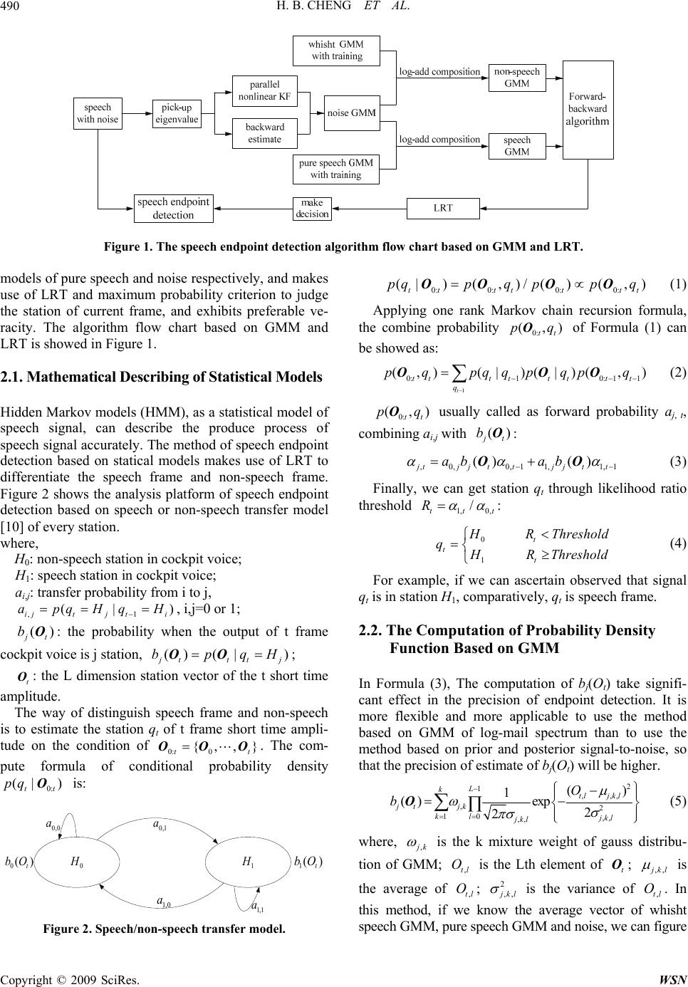

H. B. CHENG ET AL. 490
Figure 1. The speech endpoint detection algorithm flow chart based on GMM and LRT.
models of pure speech and noise respectively, and makes
use of LRT and maximum probability criterion to judge
the station of current frame, and exhibits preferable ve-
racity. The algorithm flow chart based on GMM and
LRT is showed in Figure 1.
2.1. Mathematical Describing of Statistical Models
Hidden Markov models (HMM), as a statistical model of
speech signal, can describe the produce process of
speech signal accurately. The method of speech endpoint
detection based on statical models makes use of LRT to
differentiate the speech frame and non-speech frame.
Figure 2 shows the analysis platform of speech endpoint
detection based on speech or non-speech transfer model
[10] of every station.
where,
H0: non-speech station in cockpit voice;
H1: speech station in cockpit voice;
ai,j: transfer probability from i to j,
,
(|
ijtj ti
apqHqH

 
1
)
, i,j=0 or 1;
()
jt
bO: the probability when the output of t frame
cockpit voice is j station, ()( |)
j
ttt
bpqHOO j
t
;
t
O: the L dimension station vector of the t short time
amplitude.
The way of distinguish speech frame and non-speech
is to estimate the station qt of t frame short time ampli-
tude on the condition of . The com-
pute formula of conditional probability density
is:
0: 0
{,,}
t
OOO
0:
(| )
tt
pq O
0,0
a
0,1
a
1,0
a
1,1
a
0
()
t
bO
1
()
t
bO
0
H
1
H
Figure 2. Speech/non-speech transfer model.
0: 0:0:0:
(|)( ,)/( )( ,)
tttt ttt
pqp qpp q

OOO O (1)
Applying one rank Markov chain recursion formula,
the combine probability of Formula (1) can
be showed as:
0:
(,
tt
pqO)
)
1
0:10: 11
(,)(| )(|)(,
t
ttttttt t
q
p
qpqqpqpq




OOO
)
(2)
0:
(,
tt
p
qO usually called as forward probability aj, t,
combining ai,j with ()
j
t
bO:
,0,0,11,1,
() ()
jtj jttj jtt
abab 1





OO (3)
Finally, we can get station qt through likelihood ratio
threshold 1,0,
/
tt
Rt



:
0
1
t
t
t
HR Threshold
qHR Threshold



 (4)
For example, if we can ascertain observed that signal
qt is in station H1, comparatively, qt is speech frame.
2.2. The Computation of Probability Density
Function Based on GMM
In Formula (3), The computation of bj(Ot) take signifi-
cant effect in the precision of endpoint detection. It is
more flexible and more applicable to use the method
based on GMM of log-mail spectrum than to use the
method based on prior and posterior signal-to-noise, so
that the precision of estimate of bj(Ot) will be higher.
2
1,,,
,2
10,,
,,
()
1
()exp2
2
L ktl jkl
jt jk
kljkl
jkl
O
b














O (5)
where, ,jk

is the k mixture weight of gauss distribu-
tion of GMM; is the Lth element of ;
,tl
Ot O,,
j
kl

is
the average of ;
,tl
O2
,,
j
kl
 is the variance of . In
this method, if we know the average vector of whisht
speech GMM, pure speech GMM and noise, we can figure
,tl
O

H. B. CHENG ET AL.491
out real time noise GMM and GMM with noise through
log-add composition [15] (LAC), so we can gain ()
j
t
bO
))
l
.
LAC showed as:
,,,,,, ,,,
log(1 exp(
jklS jklNlSjk
 
 (6)
where ,,,Sjkl

is the average of whisht (j=0) or speech
(j=1) GMM in log-mail spectrum, ,Nl

is the average
of noise.
In the method, we can establish whisht and pure
speech GMM by training pure speech. The average of
noise (,Nl

) can be estimated one by one frame by using
parallel nonlinear KF. The noise GMM and GMM with
noise will update timely with ,Nl

.
The traditional likelihood estimation is gained by for-
ward estimating with present and past parameter. The
value of t+1,…,T is still the important factor of time se-
quence estimate. Processing likelihood estimate with the
future frame is backward estimate. The definition of
backward estimate is:
0:0: 1:
(,)(,)( |
TttttT t
pqpqpq

OOO)
)q
(7)
Similar with Formula (2), conditional probability is
showed as:
1
1: 1
11 2:
(|)(|)
(|)( |
t
tT ttt
q
tt tT
pqpqq
pqp


 
 O
OO
1
)
t
q

(8)
1:
(|
tT t
p

O
,jt
has usually called forward probability

, combining with :
,ij
a()
jt
bO
,,0010,1,1111,
() ()1
j
titt it t
ab ab
 
 
OO

tt
pq
(9)
Usually, backward estimate begin from terminal of
tested signal, but in the test of endpoint, the terminal is
unknown. So we introduce back modularize estimation.
It is begin from T=t+b, where b is a constant. When b=0,
backward estimate equal to does not process.
We can conclude from the definition of the Forward-
Backward (F-B) algorithm that: 0: (, t H)

O
,,
j
tjt

. We can gain likelihood ratio Rt by applying
likelihood ratio test.
1, 1,
0: 1
0:00, 0,
(, )
(, )
tt
Tt
t
Ttt t
pO qH
RpO qH






 (10)
Finally, substituting Rt in Formula (4), we get the sta-
tion value qt of speech endpoint detection.
3. The Establishing of Complex Laplacian
Distribution Model
Speech endpoint detection is processed one by one frame.
Every frame includes M sampling. In generally, speech
signal is thought as windless signal in short period
(10~30ms). We can suppose that speech signal with
noise is statistical irrelated complex Laplacian random
course. We denote coefficient vector of discrete fourier
transform (DFT) of M dimension noise speech with
: ()tX
12
() [(),(),()()]
T
kM
tXtXtXt XtX=
If and
k(R)
Xk(I)
X
denote real part and imaginary
part of k
X
respectively, the probability density distri-
bution of and
k(R)
Xk(I)
X
, according to the Laplacian
probability distribution, can be written as:
k(R)
k(R)
xx
2
1
( )exp{}
X
pX

 (11)
k(I)
k(I)
xx
2
1
() exp{
X
pX


} (12)
where, 2
x

is the variance of k
X
. If the real part and
imaginary part of k
X
are uncorrelated, the distribution
density of k
X
can be written as:
kk(R) k(I)
k(R) k(I)
2
xx
() ()()
2( )
1exp{ }
pX pXpX
XX
 


 (13)
4. The Likelihood Ratio Test Based on
Hypothesis Test
Speech endpoint detection can be regarded as a binary
hypothesis issue:
0
1
:()=
:()
Hspeech donotappeartt()
=()+()
H
speech appearttt
XN
XNS
where, H0 denote the situation of speech not appearing,
Hl denote the situation of speech appearing, N(t) and S(t)
denote DFT coefficient vector of background noise and
pure speech respectively. The conditional probability
density of noise under the situation of H and Hl can be
written as:
k(R) k(I)
kn0
n,k n,k
2( )
1
(H =H )exp{}
XX
pX


 (14)
k(R) k(I)
kn 1
n,k s,kn,ks,k
2( )
1
(H=H )exp{}
XX
pX
 


(15)
We can receive likelihood test of hypothesis test by
Formulas (14) and (15). Likelihood ratio of the kth
frequency band can be denoted as:
k


H. B. CHENG ET AL. 492
kn 1
k
kn0
(H=H)
(H=H)
pX
pX
 (16)
Because the signal samples are
uncorrelated and have the same distribution, the likeli-
hood ratio of M dimension observed vector of two hy-
pothesis is:
k(1,2kX)M
 () (),,
1
1
0
0
2()(()/ )
1
()(
()(
1
1
kRkIknkknk
M
nkn
k
nkn
MXX XX
kk
pHH pXHH
PHH pXHH
e







 




X
X

1
0
)
)

(17)
where, k

is the forward signal-to-noise, define as
,
,
s
k
nk
k



, we assume that all the frequency vectors are
uncorrelated.
We can know from Formula (17) that n,k

and k

have great influence on the veracity of likelihood ratio
test. The estimate of n,k

of traditional speech endpoint
detection updates in speech intermission time. The power
spectrum changes when speech appears in cockpit voice
background, where the impulse noise does not appear in
other time. So, the estimation of noise power spectrum
should be updated really both when speech appear and
when speech do not appear. We adopt the method of long
time power spectrum smooth to compute n,k

[16].
From [16] we know that the estimation of the kth fourier
transform coefficient variance is:
2
,,
ˆˆ
(1)()(1)[()()]
nn
nknkk k
ttENt

   Xt (18)
where, is the estimation of
,
ˆ()
nk t

,() nk t

and n


is
the smooth coefficient. Considering the two situation of
speech appearing and not appearing, the estimation of the
noise power spectrum of current frame is:
2
2
00
2
11
[() ()]
[() (),](())
[() (),](()
kk
kknn k
kknn k
EN tXt
ENtX tHHPHHX t
ENtX tHHPHHXt

)
(19)
where：2
0
[() (),]()
kkn k
ENtX tHHX t 2
2
1
2
2
,
[() (),]
ˆ() 1
ˆ
()()()(
ˆˆ
1() 1()
kkn
k
nk k
kk
EN tXt HH
ttX
tt





)t
The prior signal-to-noise k

can be estimated, fol-
lowing literature [17], as:
2
,
ˆ(1)
ˆˆ
()(1)[() 1]
ˆ(1)
k
kSNRSNRk
nk
St
t
t
 


 

where, ,
,0
[] 0,
xx
Px others




2
k
k
n
X


is posterior
signal-to-noise, is it’s estimation,
ˆ()
kt

SNR

is the
weight of direct judge estimate,
2
ˆ(1)
k
St is the
speech amplitude breadth of pre-frame which has esti-
mated by using MMSE.
We can gain likelihood estimate by substituting (18)
and (20) in (7).We can judge whether speech appear or
not based on traditional MAP criterion [18].
5. The Judge Criterion Based on Conditional
MAP
The decision-making of speech endpoint detection based
on traditional MAP criterion is:
1
0
1
0
()
1
()
H
n
nH
pH H
PH H



X
X (21)
where, Hn denote the nth frame right hypothesis. Ac-
cording to Bayesian formula, the criterion of likelihood
ratio is:
1
0
10
01
()
(
()(
H
nn
nn
H
pHH pH H
PHH PHH




X
X
)
)
(22)
However, the speech appear model H1 include speech
do not appear model H0. It causes the computing of like-
lihood ratio partial to H
1 [10]. In order to make up the
difference, the Formula (22) is adjusted as:
1
0
10
01
()
()
1
()()
H
nn
nn H
pHH pH H
PHH PHH





X
X
， (23)
The speech endpoint detection of interframe has strong
relativity. The probability of that speech frame’s next
frame turns into speech frame is very large. The relativ-
ity was validated by FSM [11].
The paper combined the relativity of interframe with
MAP criterion. It is different from traditional forward
probability (
n
PH X). The present observed value and
the decision-making of pre-frame were used for comput-
ing forward probability. It was denoted as 1 (,
nn
PH H X)
,
and the decision-making verification of speech endpoint
detection decision-making was adjusted:
1
0
11
01
(,)
0,1
(,)
H
nni
nni H
pH HHHi
PH HHH







X
X (24)
P
t (20) where, α is threshold. The estimation of likelihood ratio
becomes:

H. B. CHENG ET AL.493
1
0
11
01
01
11
(,)
(,)
()
,0,
()
nni
nni
H
nni
nni H
pHHH H
PHHH H
pHH HHi
PHH HH










X
X
1
(25)
In the actual cockpit voice, because of the lack of prior
information, distributed parameters, 11 (,
nn
)
i
p
HHH H

X
and 01 (,
nn
PHHH H

X)
i
, have not been estimated,
and the distributed parameters of current frame were
decided by the current observed value. So it was predi-
gested as:
1
(,)(
0,1, 0,1.
njn inj
pHHHH PHH
ij



XX),
(26)
Formula (25) is changed to:
1
0
1
0
01
11
()
()
()
,0,
()
n
n
H
nni
nni H
pHH
PHH
pHH HHi
PHH HH








X
X
1
(27)
Its form of log is:
1
0
1
0
01
11
()
log ()
()
log, 0,1
()
n
n
H
nni
i
nni
H
pHH
PHH
pHH HHi
PHH HH












X
X


(28)
The Formula (27) or (28) is the judge criterion of
speech endpoint detection. i

is the threshold. When
preframe is speech frame, 1

will be regarded as the
threshold of the current frame. When preframe is non-
speech frame, 0

will be regarded as the threshold of
the current frame. Multiple thresholds can provide more
freedom and can enhance the robusticity of speech end-
point detection. Considering the relativity of interframe,
parameter distribution has the trait as follows:
010 011
11 0111
()(
()(
nn nn
nn nn
pHH HHpHH HH
PHH HHPHH HH


 

 
)
)


(29)
It indicates that the probability of nonspeech frame’s
next frame become nonspeech frame is large. When the
preframe is nonspeech frame, 0

is larger than 1

. It is
all the same for speech frame.
6. Experimentation
In order to test the validity of the paper’s algorithm, the
cockpit voice background sound of airplane normal sta-
tion and wrecked station have been picked up respec-
tively, and two teams experimentation of speech end-
point detection based on GMM and the paper’s algorithm
have been done.
6.1. The Establishment of Experimentation
In environment of lab, we record 200 sentences of 6
persons (3 men and 3 women) to form storage of pure
speech and training GMM. The test group makes up of
other 40 sentences. Because cockpit voice background
sound is complex, excessive, so its bandwidth is broad
(150Hz-6800Hz), and its signal is not calm and is tran-
sient. Different kind airplanes have different cockpit
voice background sounds. Its characteristics are different
from F16 noise provided by group NOISEX-2. So that,
the cockpit voice background sound used in simulation
test was recorded in the real environment. Its sample
frequency is 16KHz and quantitative change bite is 16
and single channel is format wave. We can get airplane
normal station and wrecked station speech with noise
group by adjusting breadth of pure speech and adding it
to cockpit voice background sound. The extracting of
character is showed in Table 1.
When training GMM, the GMM parameter with 25
characteristic vector (12 rank mail cepstral coefficient
and its differential coefficient, short time power differen-
tial coefficient) was gained by using the expectation-
maximization (EM) algorithm. The smooth coefficient
n


, the weight SNR

for judging forward signal-to-noise
estimation and the known threshold ηi based on preframe
should be chosen carefully to ensure the robusticity.
6.2. The Result of Experiment
We define that is the ratio that the speech frame is
detected as the speech frame correctly and is the
ratio that the nonspeech frame is detected as the speech
frame. The performance of the two algorithms is de-
picted by the ROC curve which denote the relation of
and . Figure 3 shows a real example of speech
endpoint detection. Its last time is 1s. Figure 4 and Fig-
ure 5 show the ROC curve, which is the cockpit voice
background speech endpoint detection of airplane normal
station and wrecked station, of the two algorithms.
d
P
f
P
d
Pf P
In Figure 3, the broken line of pure speech graph is the
manual mark place of speech begin point. When the air-
Table 1. the condition of character extracting.
Sample frequency 16kHz
Quantitative change bite 16bite
Advance add quantity 1-0.97z-1
Length of frame 20ms
Moving of frame 10ms
Function of window Hamming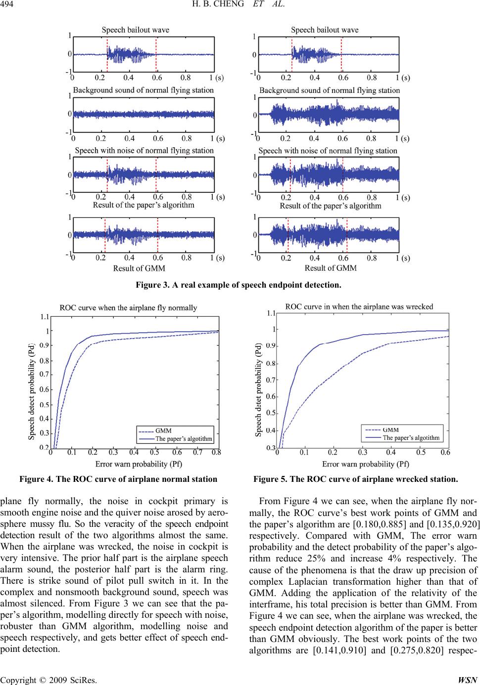

H. B. CHENG ET AL. 494
Figure 3. A real example of speech endpoint detection.
Figure 4. The ROC curve of airplane normal station Figure 5. The ROC curve of airplane wrecked station.
plane fly normally, the noise in cockpit primary is
smooth engine noise and the quiver noise arosed by aero-
sphere mussy flu. So the veracity of the speech endpoint
detection result of the two algorithms almost the same.
When the airplane was wrecked, the noise in cockpit is
very intensive. The prior half part is the airplane speech
alarm sound, the posterior half part is the alarm ring.
There is strike sound of pilot pull switch in it. In the
complex and nonsmooth background sound, speech was
almost silenced. From Figure 3 we can see that the pa-
per’s algorithm, modelling directly for speech with noise,
robuster than GMM algorithm, modelling noise and
speech respectively, and gets better effect of speech end-
point detection.
From Figure 4 we can see, when the airplane fly nor-
mally, the ROC curve’s best work points of GMM and
the paper’s algorithm are [0.180,0.885] and [0.135,0.920]
respectively. Compared with GMM, The error warn
probability and the detect probability of the paper’s algo-
rithm reduce 25% and increase 4% respectively. The
cause of the phenomena is that the draw up precision of
complex Laplacian transformation higher than that of
GMM. Adding the application of the relativity of the
interframe, his total precision is better than GMM. From
Figure 4 we can see, when the airplane was wrecked, the
speech endpoint detection algorithm of the paper is better
than GMM obviously. The best work points of the two
algorithms are [0.141,0.910] and [0.275,0.820] respec-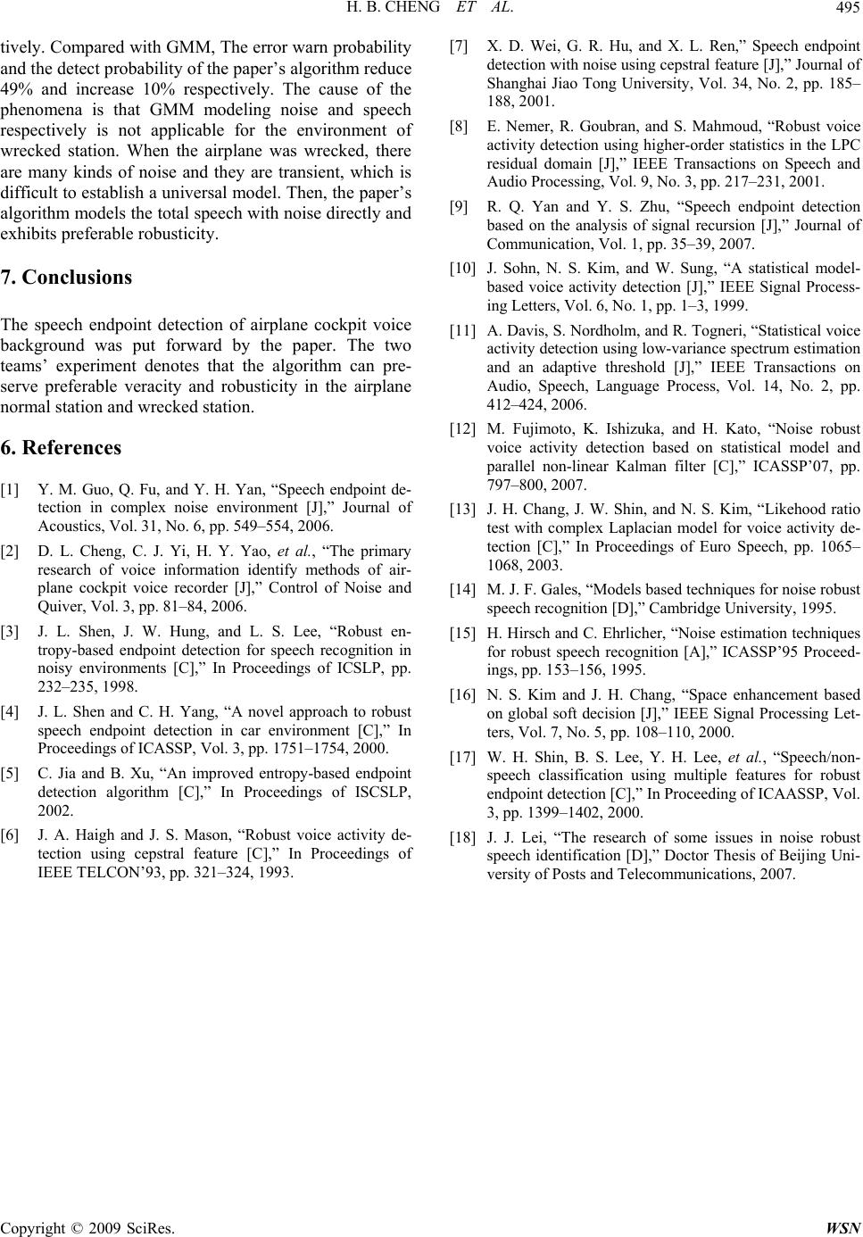

H. B. CHENG ET AL.495
tively. Compared with GMM, The error warn probability
and the detect probability of the paper’s algorithm reduce
49% and increase 10% respectively. The cause of the
phenomena is that GMM modeling noise and speech
respectively is not applicable for the environment of
wrecked station. When the airplane was wrecked, there
are many kinds of noise and they are transient, which is
difficult to establish a universal model. Then, the paper’s
algorithm models the total speech with noise directly and
exhibits preferable robusticity.
7. Conclusions
The speech endpoint detection of airplane cockpit voice
background was put forward by the paper. The two
teams’ experiment denotes that the algorithm can pre-
serve preferable veracity and robusticity in the airplane
normal station and wrecked station.
6. References
[1] Y. M. Guo, Q. Fu, and Y. H. Yan, “Speech endpoint de-
tection in complex noise environment [J],” Journal of
Acoustics, Vol. 31, No. 6, pp. 549–554, 2006.
[2] D. L. Cheng, C. J. Yi, H. Y. Yao, et al., “The primary
research of voice information identify methods of air-
plane cockpit voice recorder [J],” Control of Noise and
Quiver, Vol. 3, pp. 81–84, 2006.
[3] J. L. Shen, J. W. Hung, and L. S. Lee, “Robust en-
tropy-based endpoint detection for speech recognition in
noisy environments [C],” In Proceedings of ICSLP, pp.
232–235, 1998.
[4] J. L. Shen and C. H. Yang, “A novel approach to robust
speech endpoint detection in car environment [C],” In
Proceedings of ICASSP, Vol. 3, pp. 1751–1754, 2000.
[5] C. Jia and B. Xu, “An improved entropy-based endpoint
detection algorithm [C],” In Proceedings of ISCSLP,
2002.
[6] J. A. Haigh and J. S. Mason, “Robust voice activity de-
tection using cepstral feature [C],” In Proceedings of
IEEE TELCON’93, pp. 321–324, 1993.
[7] X. D. Wei, G. R. Hu, and X. L. Ren,” Speech endpoint
detection with noise using cepstral feature [J],” Journal of
Shanghai Jiao Tong University, Vol. 34, No. 2, pp. 185–
188, 2001.
[8] E. Nemer, R. Goubran, and S. Mahmoud, “Robust voice
activity detection using higher-order statistics in the LPC
residual domain [J],” IEEE Transactions on Speech and
Audio Processing, Vol. 9, No. 3, pp. 217–231, 2001.
[9] R. Q. Yan and Y. S. Zhu, “Speech endpoint detection
based on the analysis of signal recursion [J],” Journal of
Communication, Vol. 1, pp. 35–39, 2007.
[10] J. Sohn, N. S. Kim, and W. Sung, “A statistical model-
based voice activity detection [J],” IEEE Signal Process-
ing Letters, Vol. 6, No. 1, pp. 1–3, 1999.
[11] A. Davis, S. Nordholm, and R. Togneri, “Statistical voice
activity detection using low-variance spectrum estimation
and an adaptive threshold [J],” IEEE Transactions on
Audio, Speech, Language Process, Vol. 14, No. 2, pp.
412–424, 2006.
[12] M. Fujimoto, K. Ishizuka, and H. Kato, “Noise robust
voice activity detection based on statistical model and
parallel non-linear Kalman filter [C],” ICASSP’07, pp.
797–800, 2007.
[13] J. H. Chang, J. W. Shin, and N. S. Kim, “Likehood ratio
test with complex Laplacian model for voice activity de-
tection [C],” In Proceedings of Euro Speech, pp. 1065–
1068, 2003.
[14] M. J. F. Gales, “Models based techniques for noise robust
speech recognition [D],” Cambridge University, 1995.
[15] H. Hirsch and C. Ehrlicher, “Noise estimation techniques
for robust speech recognition [A],” ICASSP’95 Proceed-
ings, pp. 153–156, 1995.
[16] N. S. Kim and J. H. Chang, “Space enhancement based
on global soft decision [J],” IEEE Signal Processing Let-
ters, Vol. 7, No. 5, pp. 108–110, 2000.
[17] W. H. Shin, B. S. Lee, Y. H. Lee, et al., “Speech/non-
speech classification using multiple features for robust
endpoint detection [C],” In Proceeding of ICAASSP, Vol.
3, pp. 1399–1402, 2000.
[18] J. J. Lei, “The research of some issues in noise robust
speech identification [D],” Doctor Thesis of Beijing Uni-
versity of Posts and Telecommunications, 2007.