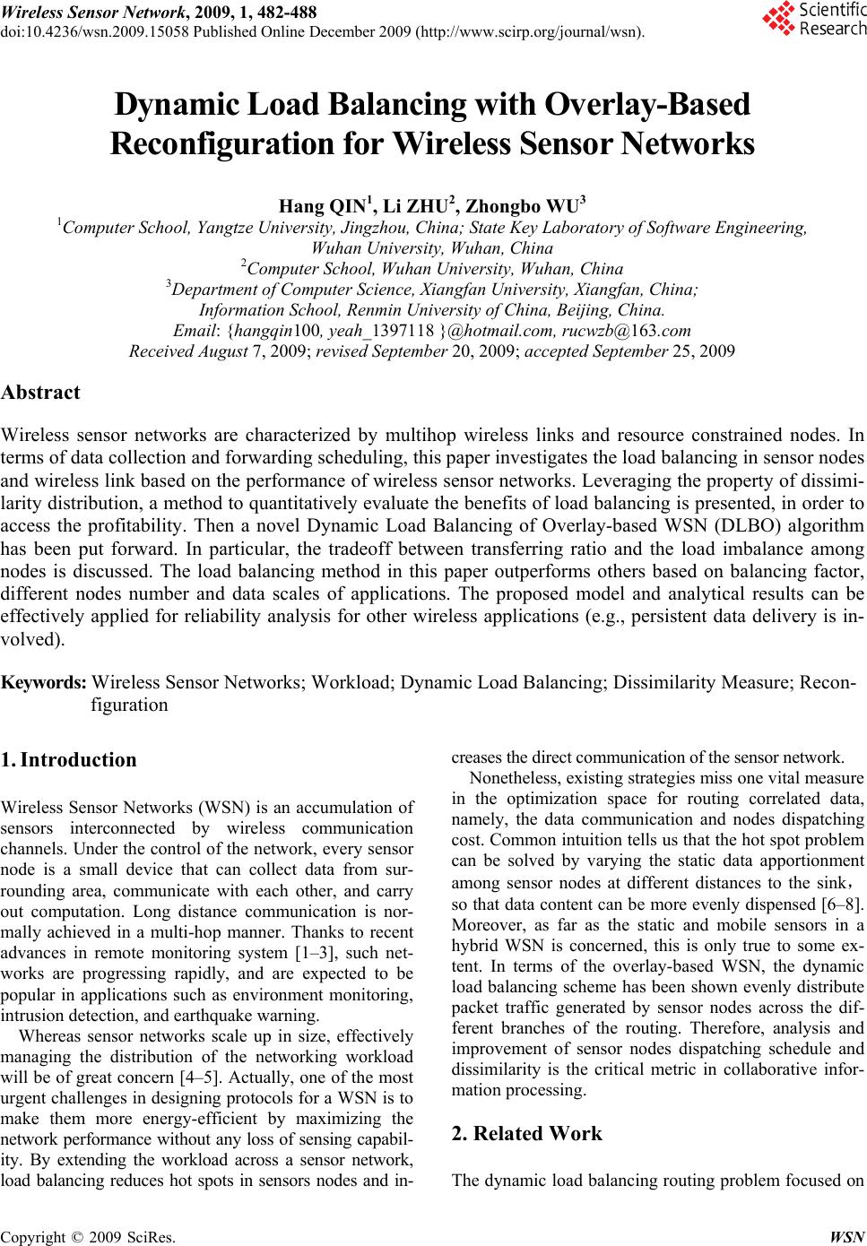Wireless Sensor Network, 2009, 1, 482-488
doi:10.4236/wsn.2009.15058 Published Online December 2009 (http://www.scirp.org/journal/wsn).
Dynamic Load Balancing with Overlay-Based
Reconfiguration for Wireless Sensor Networks
Hang QIN1, Li ZHU2, Zhongbo WU3
1Computer School, Yangtze University, Jingzhou, China; State Key Laboratory of Software Engineering,
Wuhan University, Wuhan, China
2Computer School, Wuhan University, Wuhan, China
3Department of Computer Science, Xiangfan University, Xiangfan, China;
Information School, Renmin University of China, Beijing, China.
Received August 7, 2009; revised September 20, 2009; accepted September 25, 2009
Abstract
Wireless sensor networks are characterized by multihop wireless links and resource constrained nodes. In
terms of data collection and forwarding scheduling, this paper investigates the load balancing in sensor nodes
and wireless link based on the performance of wireless sensor networks. Leveraging the property of dissimi-
larity distribution, a method to quantitatively evaluate the benefits of load balancing is presented, in order to
access the profitability. Then a novel Dynamic Load Balancing of Overlay-based WSN (DLBO) algorithm
has been put forward. In particular, the tradeoff between transferring ratio and the load imbalance among
nodes is discussed. The load balancing method in this paper outperforms others based on balancing factor,
different nodes number and data scales of applications. The proposed model and analytical results can be
effectively applied for reliability analysis for other wireless applications (e.g., persistent data delivery is in-
volved).
Keywords: Wireless Sensor Networks; Workload; Dynamic Load Balancing; Dissimilarity Measure; Recon-
figuration
1. Introduction
Wireless Sensor Networks (WSN) is an accumulation of
sensors interconnected by wireless communication
channels. Under the control of the network, every sensor
node is a small device that can collect data from sur-
rounding area, communicate with each other, and carry
out computation. Long distance communication is nor-
mally achieved in a multi-hop manner. Thanks to recent
advances in remote monitoring system [1–3], such net-
works are progressing rapidly, and are expected to be
popular in applications such as environment monitoring,
intrusion detection, and earthquake warning.
Whereas sensor networks scale up in size, effectively
managing the distribution of the networking workload
will be of great concern [4–5]. Actually, one of the most
urgent challenges in designing protocols for a WSN is to
make them more energy-efficient by maximizing the
network performance without any loss of sensing capabil-
ity. By extending the workload across a sensor network,
load balancing reduces hot spots in sensors nodes and in-
creases the direct communication of the sensor network.
Nonetheless, existing strategies miss one vital measure
in the optimization space for routing correlated data,
namely, the data communication and nodes dispatching
cost. Common intuition tells us that the hot spot problem
can be solved by varying the static data apportionment
among sensor nodes at different distances to the sink，
so that data content can be more evenly dispensed [6–8].
Moreover, as far as the static and mobile sensors in a
hybrid WSN is concerned, this is only true to some ex-
tent. In terms of the overlay-based WSN, the dynamic
load balancing scheme has been shown evenly distribute
packet traffic generated by sensor nodes across the dif-
ferent branches of the routing. Therefore, analysis and
improvement of sensor nodes dispatching schedule and
dissimilarity is the critical metric in collaborative infor-
mation processing.
2. Related Work
The dynamic load balancing routing problem focused on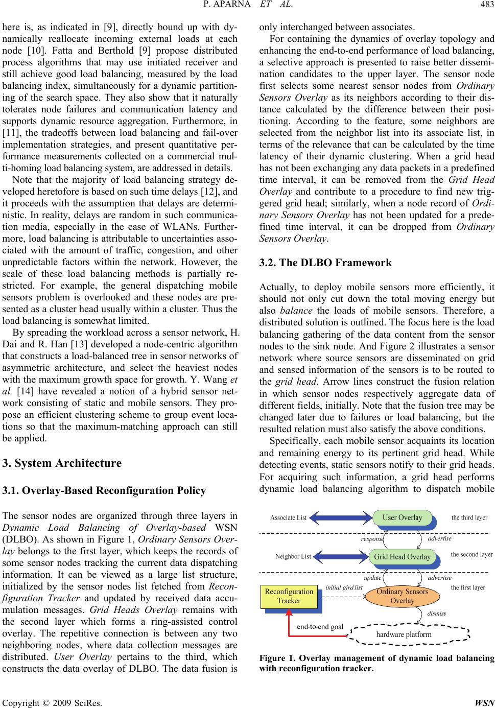

P. APARNA ET AL.483
here is, as indicated in [9], directly bound up with dy-
namically reallocate incoming external loads at each
node [10]. Fatta and Berthold [9] propose distributed
process algorithms that may use initiated receiver and
still achieve good load balancing, measured by the load
balancing index, simultaneously for a dynamic partition-
ing of the search space. They also show that it naturally
tolerates node failures and communication latency and
supports dynamic resource aggregation. Furthermore, in
[11], the tradeoffs between load balancing and fail-over
implementation strategies, and present quantitative per-
formance measurements collected on a commercial mul-
ti-homing load balancing system, are addressed in details.
Note that the majority of load balancing strategy de-
veloped heretofore is based on such time delays [12], and
it proceeds with the assumption that delays are determi-
nistic. In reality, delays are random in such communica-
tion media, especially in the case of WLANs. Further-
more, load balancing is attributable to uncertainties asso-
ciated with the amount of traffic, congestion, and other
unpredictable factors within the network. However, the
scale of these load balancing methods is partially re-
stricted. For example, the general dispatching mobile
sensors problem is overlooked and these nodes are pre-
sented as a cluster head usually within a cluster. Thus the
load balancing is somewhat limited.
By spreading the workload across a sensor network, H.
Dai and R. Han [13] developed a node-centric algorithm
that constructs a load-balanced tree in sensor networks of
asymmetric architecture, and select the heaviest nodes
with the maximum growth space for growth. Y. Wang et
al. [14] have revealed a notion of a hybrid sensor net-
work consisting of static and mobile sensors. They pro-
pose an efficient clustering scheme to group event loca-
tions so that the maximum-matching approach can still
be applied.
3. System Architecture
3.1. Overlay-Based Reconfiguration Policy
The sensor nodes are organized through three layers in
Dynamic Load Balancing of Overlay-based WSN
(DLBO). As shown in Figure 1, Ordinary Sensors Over-
lay belongs to the first layer, which keeps the records of
some sensor nodes tracking the current data dispatching
information. It can be viewed as a large list structure,
initialized by the sensor nodes list fetched from Recon-
figuration Tracker and updated by received data accu-
mulation messages. Grid Heads Overlay remains with
the second layer which forms a ring-assisted control
overlay. The repetitive connection is between any two
neighboring nodes, where data collection messages are
distributed. User Overlay pertains to the third, which
constructs the data overlay of DLBO. The data fusion is
only interchanged between associates.
For containing the dynamics of overlay topology and
enhancing the end-to-end performance of load balancing,
a selective approach is presented to raise better dissemi-
nation candidates to the upper layer. The sensor node
first selects some nearest sensor nodes from Ordinary
Sensors Overlay as its neighbors according to their dis-
tance calculated by the difference between their posi-
tioning. According to the feature, some neighbors are
selected from the neighbor list into its associate list, in
terms of the relevance that can be calculated by the time
latency of their dynamic clustering. When a grid head
has not been exchanging any data packets in a predefined
time interval, it can be removed from the Grid Head
Overlay and contribute to a procedure to find new trig-
gered grid head; similarly, when a node record of Ordi-
nary Sensors Overlay has not been updated for a prede-
fined time interval, it can be dropped from Ordinary
Sensors Overlay.
3.2. The DLBO Framework
Actually, to deploy mobile sensors more efficiently, it
should not only cut down the total moving energy but
also balance the loads of mobile sensors. Therefore, a
distributed solution is outlined. The focus here is the load
balancing gathering of the data content from the sensor
nodes to the sink node. And Figure 2 illustrates a sensor
network where source sensors are disseminated on grid
and sensed information of the sensors is to be routed to
the grid head. Arrow lines construct the fusion relation
in which sensor nodes respectively aggregate data of
different fields, initially. Note that the fusion tree may be
changed later due to failures or load balancing, but the
resulted relation must also satisfy the above conditions.
Specifically, each mobile sensor acquaints its location
and remaining energy to its pertinent grid head. While
detecting events, static sensors notify to their grid heads.
For acquiring such information, a grid head performs
dynamic load balancing algorithm to dispatch mobile
Figure 1. Overlay management of dynamic load balancing
with reconfiguration tracker.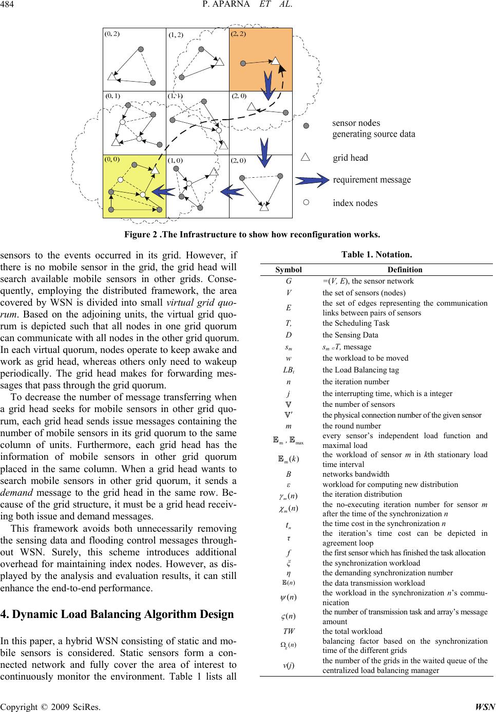

P. APARNA ET AL. 484
Figure 2 .The Infrastructure to show how reconfiguration works.
sensors to the events occurred in its grid. However, if
there is no mobile sensor in the grid, the grid head will
search available mobile sensors in other grids. Conse-
quently, employing the distributed framework, the area
covered by WSN is divided into small virtual grid quo-
rum. Based on the adjoining units, the virtual grid quo-
rum is depicted such that all nodes in one grid quorum
can communicate with all nodes in the other grid quorum.
In each virtual quorum, nodes operate to keep awake and
work as grid head, whereas others only need to wakeup
periodically. The grid head makes for forwarding mes-
sages that pass through the grid quorum.
Table 1. Notation.
Symbol Definition
G =(V, E), the sensor network
V the set of sensors (nodes)
E the set of edges representing the communication
links between pairs of sensors
T, the Scheduling Task
D the Sensing Data
sm sm
∈
T, message
w the workload to be moved
LBt the Load Balancing tag
n the iteration number
j the interrupting time, which is a integer
To decrease the number of message transferring when
a grid head seeks for mobile sensors in other grid quo-
rum, each grid head sends issue messages containing the
number of mobile sensors in its grid quorum to the same
column of units. Furthermore, each grid head has the
information of mobile sensors in other grid quorum
placed in the same column. When a grid head wants to
search mobile sensors in other grid quorum, it sends a
demand message to the grid head in the same row. Be-
cause of the grid structure, it must be a grid head receiv-
ing both issue and demand messages.

the number of sensors


the physical connection number of the given sensor
m the round number
m
 max 
m()k
, every sensor’s independent load function and
maximal load
the workload of sensor m in kth stationary load
time interval
B networks bandwidth
ε workload for computing new distribution
()
n
m

the iteration distribution
()
mn
 the no-executing iteration number for sensor m
after the time of the synchronization n
This framework avoids both unnecessarily removing
the sensing data and flooding control messages through-
out WSN. Surely, this scheme introduces additional
overhead for maintaining index nodes. However, as dis-
played by the analysis and evaluation results, it can still
enhance the end-to-end performance.
n
t
()n
()n
the time cost in the synchronization n
τ the iteration’s time cost can be depicted in
agreement loop
f the first sensor which has finished the task allocation
ξ the synchronization workload
η the demanding synchronization number
the data transmission workload

the workload in the synchronization n’s commu-
nication
4. Dynamic Load Balancing Algorithm Design ()n

the number of transmission task and array’s message
amount
TW the total workload
In this paper, a hybrid WSN consisting of static and mo-
bile sensors is considered. Static sensors form a con-
nected network and fully cover the area of interest to
continuously monitor the environment. Table 1 lists all
()
gn balancing factor based on the synchronization
time of the different grids
v(j) the number of the grids in the waited queue of the
centralized load balancing manager

P. APARNA ET AL.485
notation in this paper, and the problem of dispatching
mobile sensors is modeled in Table 1.
The sensor network is modeled as a graph G=(V, E),
where V denotes the set of sensors (nodes) and E the set
of edges representing the communication links between
pairs of sensors. The dynamic load balancing architec-
ture is executed on G to construct a load-balanced tree.
The load associated with a given sensor node represents
the amount of data periodically generated by that sensor
node. Actually, the above framework absorbs the nodes
generating the greatest load to the lightest branches to
achieve balance.
The study identifies the Dynamic policy in DLBO, it
is composed of a Scheduling Server’s Algorithm and a
Task Counter’s Algorithm. Firstly, Scheduling Server’s
Algorithm derives a task and divides sensing data to
every task equally. The algorithms are detailed below for
the sake of completeness:
Epoch 1: Scheduling Server’s Algorithm
Initialization:
1. derive T to every sensor node, and equally allocate
D into the set of T, where T is Scheduling Task, D is
Sensing Data
Iteration:
2. receive any message from sm, sm ∈ T;
3. if (message∈workload’s neighboring information)
then fill in corresponding overlay;
4. if(wm= 0) then
5. search hotspot task sm by MAX{t1, t2,. . . };
6. get the sensing data’s size
7. if (w match the tradeoff condition) then
8. mount LBt
9. send( LBt, sn, w) to sn;r
10. interrupt sn, send(sn, w) to sn;
11. if (T is Null) then exit, all task has been finished.
Secondly, while one task has been finished, Task
Counter’s Algorithm can get the condition and granular-
ity of load balancing from the Task’s optimal size.
Epoch 2: Task Counter’s Algorithm
1. interrupt initialization, set interrupting time, j ← 0;
2. if(j<=uptoround－1) then
3. sensors nodes’ data transferring part
4. if(j= =uptoround－1) then
5. send workload information to Scheduler, return load
balancing parameters;
6. receive LBt, sn and w;
7. if (LBt trigger scheduling) then
8. receive w packets from sn;
9. uptoround ← w;
10. update node’s data distribution;
11. i←i＋1;
12. goto (2);
13. send task’s finishing information to the scheduler.
Finally, the Interrupting Procedure is as follows:
Epoch 3: Interrupting Procedure
1. receive message w from scheduler;
2. send w packets to task ni;
3. uptoround ← uptoround－l;
4. update the sensor node’s data distribution.
5. Workload Analysis with Data
Communication
In this paper, the workload model is developed in order
to examine the effect for load balancing strategy. One
strategy’s workload is primarily composed of these four
parts:
 Workload for Computing New Distribution
 Synchronization Workload
 Workload for Data communication
 Workload for Dispatching Sensors

denote the number of sensors, where Let


is the
physical connection number of the given sensor, and m is
round number, n is iteration number. Let be every
sensor’s independent load function,is every sensor’s
maximal load, is the workload of sensor m in kth
stationary load time interval, and B is networks band-
width.
m

max

m()k
Firstly, as far as Workload for Computing New Dis-
tribution is concerned, workload can be defined by

,
and normally it is a small quantum. In this distributed
strategy, every sensor node has the cost. Moreover, the
workload is relatively smaller in the local strategy be-
cause of


nodes in the grid event locations, and this
difference can be ignored.
Secondly, Synchronization Workload is the hotspot
node forwards interrupting request to the neighboring
nodes in the synchronization process, which conse-
quently reflects their performance and energy parameters
to the reconfiguration tracker for load balancing. The
workload can be calculated in terms of the category of
data aggregation.
5.1. Definition 1: Workload for Dispatching
Sensors
The demanding message number can be analyzed ac-
cording to data transmission and sensors rescheduling.
The iteration distribution can be identified as , and
()
mn

()
mn

defines the no-executing iteration number for
sensor m after the time of the synchronization n.
1 () () m nm
n 




, and depicts the time cost in the syn-
chronization n.
n
t
Based on the influence of discrete workload, the sen-
sor’s effective speed is in the inverse proportion to the
sensor’s workload, thus the computation expression is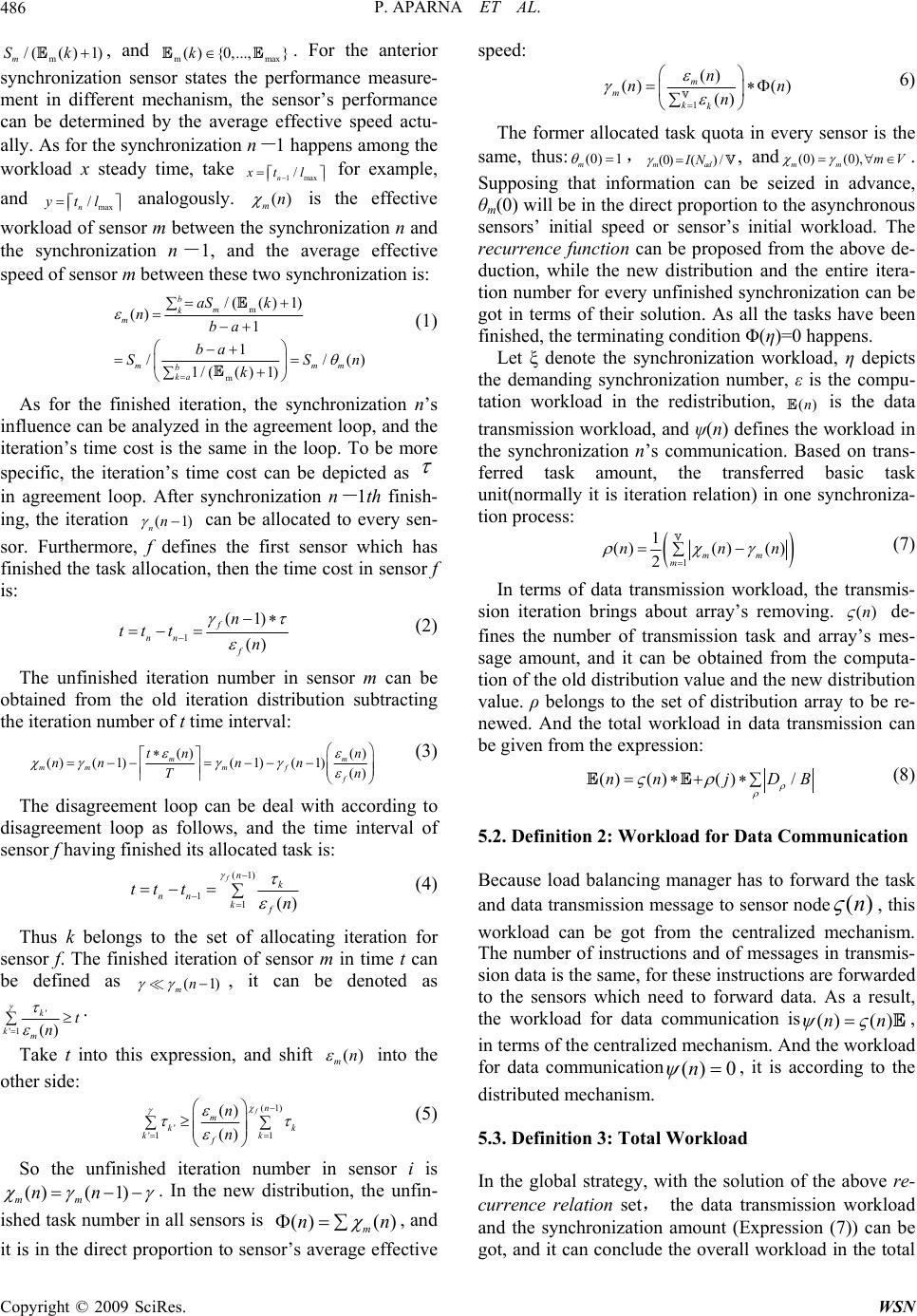

P. APARNA ET AL. 486
/(
m
Smmax ) {0,...,}k
1max
/
n
xt l



maxn()
mn
m( )1)k (
/ytl

, and . For the anterior
synchronization sensor states the performance measure-
ment in different mechanism, the sensor’s performance
can be determined by the average effective speed actu-
ally. As for the synchronization n － 1 happens among the
workload x steady time, take for example,
and analogously.

is the effective
workload of sensor m between the synchronization n and
the synchronization n － 1, and the average effective
speed of sensor m between these two synchronization is:
m
m
/((
() 1
1
1/(( )
b
m k
m
b
ka
aS
nba
ba
k









) 1)
// ()
1)
mm
m
k
SSn 





(1)
As for the finished iteration, the synchronization n’s
influence can be analyzed in the agreement loop, and the
iteration’s time cost is the same in the loop. To be more
specific, the iteration’s time cost can be depicted as

in agreement loop. After synchronization n － 1th finish-
ing, the iteration (1)
nn

 can be allocated to every sen-
sor. Furthermore, f defines the first sensor which has
finished the task allocation, then the time cost in sensor f
is:
1nn
tt t(1)
()
f
f
n
n






 (2)
The unfinished iteration number in sensor m can be
obtained from the old iteration distribution subtracting
the iteration number of t time interval:
()
() (1)(1)
m
mm m
tn
nn n

 



 


()
(1) ()
m
f
f
n
n
Tn







(3)
The disagreement loop can be deal with according to
disagreement loop as follows, and the time interval of
sensor f having finished its allocated task is:
(1)
1()
fn
k
kfn

1nn
tt t






(1)
mn

 (4)
Thus k belongs to the set of allocating iteration for
sensor f. The finished iteration of sensor m in time t can
be defined as

, it can be denoted as
'
()
k
m
t
n
'1k






()
mn
.
Take t into this expression, and shift

into the
other side:
(1)
1
()
()
fn
m
kk
kk
f
n
n


'
'1







 


( 1)
mm
nn
 (5)
So the unfinished iteration number in sensor i is
()

 
() ()
m
nn

. In the new distribution, the unfin-
ished task number in all sensors is


, and
it is in the direct proportion to sensor’s average effective
speed:
1
()
() ()
()
m
m
kk
n
nn
n









(0) 1
m
6)
The former allocated task quota in every sensor is the
same, thus:

，

(0)()/
mad
IN


(0) (0),
mm
mV  
()n
, and.
Supposing that information can be seized in advance,
θm(0) will be in the direct proportion to the asynchronous
sensors’ initial speed or sensor’s initial workload. The
recurrence function can be proposed from the above de-
duction, while the new distribution and the entire itera-
tion number for every unfinished synchronization can be
got in terms of their solution. As all the tasks have been
finished, the terminating condition Φ(η)=0 happens.
Let ξ denote the synchronization workload, η depicts
the demanding synchronization number, ε is the compu-
tation workload in the redistribution, is the data
transmission workload, and ψ(n) defines the workload in
the synchronization n’s communication. Based on trans-
ferred task amount, the transferred basic task
unit(normally it is iteration relation) in one synchroniza-
tion process:


1
1
()() ()
2mm
m
nnn 




()n
(7)
In terms of data transmission workload, the transmis-
sion iteration brings about array’s removing.

de-
fines the number of transmission task and array’s mes-
sage amount, and it can be obtained from the computa-
tion of the old distribution value and the new distribution
value. ρ belongs to the set of distribution array to be re-
newed. And the total workload in data transmission can
be given from the expression:
() ()()/nn jDB


 

 
()n
(8)
5.2. Definition 2: Workload for Data Communication
Because load balancing manager has to forward the task
and data transmission message to sensor node

, this
workload can be got from the centralized mechanism.
The number of instructions and of messages in transmis-
sion data is the same, for these instructions are forwarded
to the sensors which need to forward data. As a result,
the workload for data communication is()()nn


 
() 0n

,
in terms of the centralized mechanism. And the workload
for data communication

, it is according to the
distributed mechanism.
5.3. Definition 3: Total Workload
In the global strategy, with the solution of the above re-
currence relation set， the data transmission workload
and the synchronization amount (Expression (7)) can be
got, and it can conclude the overall workload in the total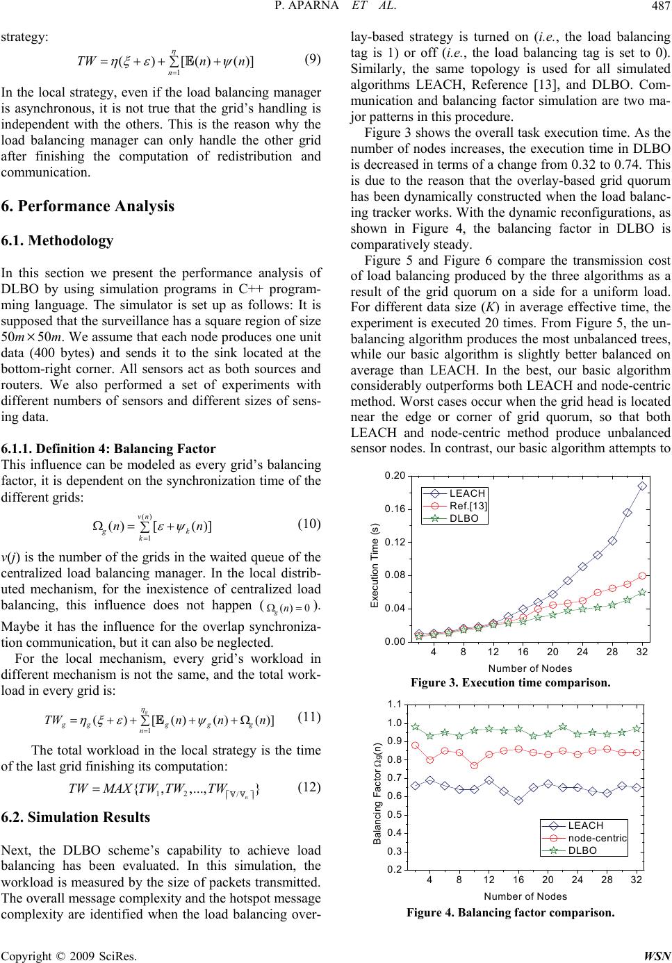

P. APARNA ET AL.487
[()()]n n  

()
1
[ ()]
vn
gk
k
nn 


() 0
gn
strategy:
1
()
n
TW

 


 (9)
In the local strategy, even if the load balancing manager
is asynchronous, it is not true that the grid’s handling is
independent with the others. This is the reason why the
load balancing manager can only handle the other grid
after finishing the computation of redistribution and
communication.
6. Performance Analysis
6.1. Methodology
In this section we present the performance analysis of
DLBO by using simulation programs in C++ program-
ming language. The simulator is set up as follows: It is
supposed that the surveillance has a square region of size
50m50m. We assume that each node produces one unit
data (400 bytes) and sends it to the sink located at the
bottom-right corner. All sensors act as both sources and
routers. We also performed a set of experiments with
different numbers of sensors and different sizes of sens-
ing data.
6.1.1. Definition 4: Balancing Factor
This influence can be modeled as every grid’s balancing
factor, it is dependent on the synchronization time of the
different grids:
() (10)
v(j) is the number of the grids in the waited queue of the
centralized load balancing manager. In the local distrib-
uted mechanism, for the inexistence of centralized load
balancing, this influence does not happen (


()()]
g g
n n   
/
,...,}
n
TW


4812 16 20 24 28 32
0.00
0.04
0.08
0.12
0.16
0.20
).
Maybe it has the influence for the overlap synchroniza-
tion communication, but it can also be neglected.
For the local mechanism, every grid’s workload in
different mechanism is not the same, and the total work-
load in every grid is:
1
()[()
g
gg g
n
TW n

 


 (11)
The total workload in the local strategy is the time
of the last grid finishing its computation:
12
{,TWMAXTWTW (12)
6.2. Simulation Results
Next, the DLBO scheme’s capability to achieve load
balancing has been evaluated. In this simulation, the
workload is measured by the size of packets transmitted.
The overall message complexity and the hotspot message
complexity are identified when the load balancing over-
lay-based strategy is turned on (i.e., the load balancing
tag is 1) or off (i.e., the load balancing tag is set to 0).
Similarly, the same topology is used for all simulated
algorithms LEACH, Reference [13], and DLBO. Com-
munication and balancing factor simulation are two ma-
jor patterns in this procedure.
Figure 3 shows the overall task execution time. As the
number of nodes increases, the execution time in DLBO
is decreased in terms of a change from 0.32 to 0.74. This
is due to the reason that the overlay-based grid quorum
has been dynamically constructed when the load balanc-
ing tracker works. With the dynamic reconfigurations, as
shown in Figure 4, the balancing factor in DLBO is
comparatively steady.
Figure 5 and Figure 6 compare the transmission cost
of load balancing produced by the three algorithms as a
result of the grid quorum on a side for a uniform load.
For different data size (K) in average effective time, the
experiment is executed 20 times. From Figure 5, the un-
balancing algorithm produces the most unbalanced trees,
while our basic algorithm is slightly better balanced on
average than LEACH. In the best, our basic algorithm
considerably outperforms both LEACH and node-centric
method. Worst cases occur when the grid head is located
near the edge or corner of grid quorum, so that both
LEACH and node-centric method produce unbalanced
sensor nodes. In contrast, our basic algorithm attempts to
Execution Time (s)
Number of Nodes
LEACH
Ref.[13]
DLBO
481216 2024 2832
0.2
0.3
0.4
0.5
0.6
0.7
0.8
0.9
1.0
1.1
Figure 3. Execution time comparison.
Balancing Factor g(n)
Number of Nodes
LEACH
node-centric
DLBO
Figure 4. Balancing factor comparison.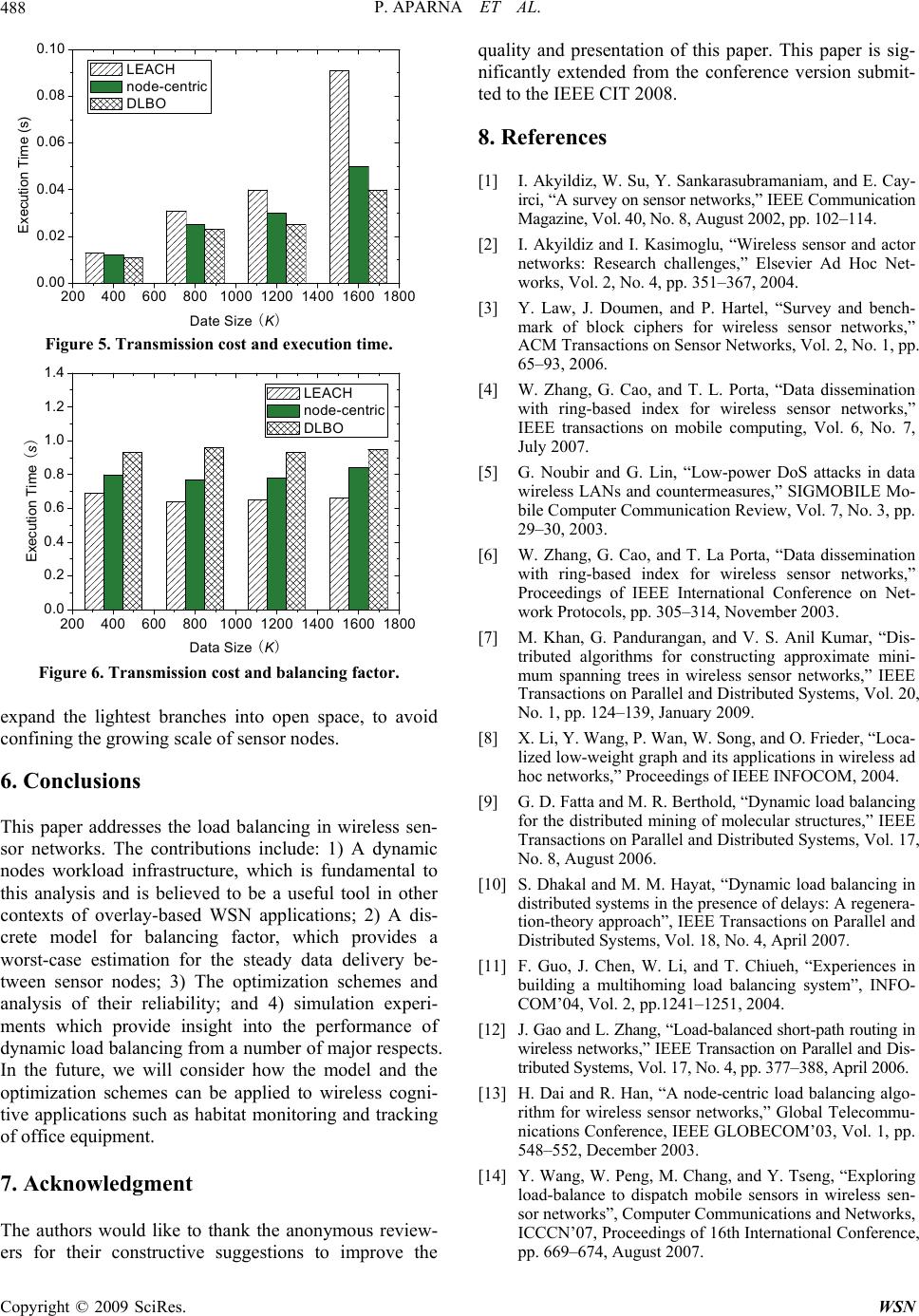

P. APARNA ET AL. 488
200 400 600 800100012001400
0.00
0.02
0.04
0.06
0.08
0.10
1600 1800
Execution Time (s)
Date Size (K)
LEACH
node-centric
DLBO
Figure 5. Transmission cost and execution time.
200 400 600 80010001200
0.0
0.2
0.4
0.6
0.8
1.0
1.2
1.4
1400 1600 1800
Execution Time (s)
Data Size (K)
LEACH
node-centric
DLBO
ers for their constructive suggestions to improve the
. References
] I. Akyildiz, W. Su, Y. Sankarasubramaniam, and E. Cay-
vey and bench-
Cao, and T. L. Porta, “Data dissemination
nd G. Lin, “Low-power DoS attacks in data
Cao, and T. La Porta, “Data dissemination
ar, “Dis-
d O. Frieder, “Loca-
g
Hayat, “Dynamic load balancing in
ences in
rt-path routing in
, “Exploring
pp. 669–674, August 2007.
Figure 6. Transmission cost and balancing factor.
expand the lightest branches into open space, to avoid
confining the growing scale of sensor nodes.
6. Conclusions
This paper addresses the load balancing in wireless sen-
sor networks. The contributions include: 1) A dynamic
nodes workload infrastructure, which is fundamental to
this analysis and is believed to be a useful tool in other
contexts of overlay-based WSN applications; 2) A dis-
crete model for balancing factor, which provides a
worst-case estimation for the steady data delivery be-
tween sensor nodes; 3) The optimization schemes and
analysis of their reliability; and 4) simulation experi-
ments which provide insight into the performance of
dynamic load balancing from a number of major respects.
In the future, we will consider how the model and the
optimization schemes can be applied to wireless cogni-
tive applications such as habitat monitoring and tracking
of office equipment.
7. Acknowledgment
The authors would like to thank the anonymous review-
quality and presentation of this paper. This paper is sig-
nificantly extended from the conference version submit-
ted to the IEEE CIT 2008.
8
[1
irci, “A survey on sensor networks,” IEEE Communication
Magazine, Vol. 40, No. 8, August 2002, pp. 102–114.
[2] I. Akyildiz and I. Kasimoglu, “Wireless sensor and actor
networks: Research challenges,” Elsevier Ad Hoc Net-
works, Vol. 2, No. 4, pp. 351–367, 2004.
[3] Y. Law, J. Doumen, and P. Hartel, “Sur
mark of block ciphers for wireless sensor networks,”
ACM Transactions on Sensor Networks, Vol. 2, No. 1, pp.
65–93, 2006.
[4] W. Zhang, G.
with ring-based index for wireless sensor networks,”
IEEE transactions on mobile computing, Vol. 6, No. 7,
July 2007.
[5] G. Noubir a
wireless LANs and countermeasures,” SIGMOBILE Mo-
bile Computer Communication Review, Vol. 7, No. 3, pp.
29–30, 2003.
[6] W. Zhang, G.
with ring-based index for wireless sensor networks,”
Proceedings of IEEE International Conference on Net-
work Protocols, pp. 305–314, November 2003.
[7] M. Khan, G. Pandurangan, and V. S. Anil Kum
tributed algorithms for constructing approximate mini-
mum spanning trees in wireless sensor networks,” IEEE
Transactions on Parallel and Distributed Systems, Vol. 20,
No. 1, pp. 124–139, January 2009.
[8] X. Li, Y. Wang, P. Wan, W. Song, an
lized low-weight graph and its applications in wireless ad
hoc networks,” Proceedings of IEEE INFOCOM, 2004.
[9] G. D. Fatta and M. R. Berthold, “Dynamic load balancin
for the distributed mining of molecular structures,” IEEE
Transactions on Parallel and Distributed Systems, Vol. 17,
No. 8, August 2006.
[10] S. Dhakal and M. M.
distributed systems in the presence of delays: A regenera-
tion-theory approach”, IEEE Transactions on Parallel and
Distributed Systems, Vol. 18, No. 4, April 2007.
[11] F. Guo, J. Chen, W. Li, and T. Chiueh, “Experi
building a multihoming load balancing system”, INFO-
COM’04, Vol. 2, pp.1241–1251, 2004.
[12] J. Gao and L. Zhang, “Load-balanced sho
wireless networks,” IEEE Transaction on Parallel and Dis-
tributed Systems, Vol. 17, No. 4, pp. 377–388, April 2006.
[13] H. Dai and R. Han, “A node-centric load balancing algo-
rithm for wireless sensor networks,” Global Telecommu-
nications Conference, IEEE GLOBECOM’03, Vol. 1, pp.
548–552, December 2003.
[14] Y. Wang, W. Peng, M. Chang, and Y. Tseng
load-balance to dispatch mobile sensors in wireless sen-
sor networks”, Computer Communications and Networks,
ICCCN’07, Proceedings of 16th International Conference,