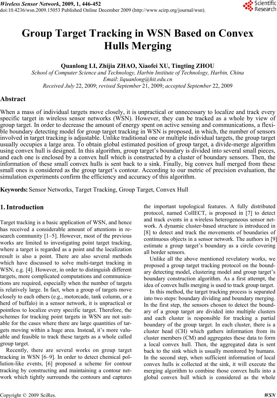Wireless Sensor Network, 2009, 1, 446-452
doi:10.4236/wsn.2009.15053 Published Online December 2009 (http://www.scirp.org/journal/wsn).
Group Target Tracking in WSN Based on Convex
Hulls Merging
Quanlong LI, Zhijia ZHAO, Xiaofei XU, Tingting ZHOU
School of Computer Science and Technology, Harbin Institute of Technology, Harbin, China
Received July 22, 2009; revised September 21, 2009; accepted September 22, 2009
Abstract
When a mass of individual targets move closely, it is unpractical or unnecessary to localize and track every
specific target in wireless sensor networks (WSN). However, they can be tracked as a whole by view of
group target. In order to decrease the amount of energy spent on active sensing and communications, a flexi-
ble boundary detecting model for group target tracking in WSN is proposed, in which, the number of sensors
involved in target tracking is adjustable. Unlike traditional one or multiple individual targets, the group target
usually occupies a large area. To obtain global estimated position of group target, a divide-merge algorithm
using convex hull is designed. In this algorithm, group target’s boundary is divided into several small pieces,
and each one is enclosed by a convex hull which is constructed by a cluster of boundary sensors. Then, the
information of these small convex hulls is sent back to a sink. Finally, big convex hull merged from these
small ones is considered as the group target’s contour. According to our metric of precision evaluation, the
simulation experiments confirm the efficiency and accuracy of this algorithm.
Keywords: Sensor Networks, Target Tracking, Group Target, Convex Hull
1. Introduction
Target tracking is a basic application of WSN, and hence
has received a considerable amount of attentions in re-
search community [1–5]. However, most of the previous
works are limited to investigating point target tracking,
where a target is regarded as a point and the localization
result is also a point. There are also several methods
which have discussed to solve multi-target tracking in
WSN, e.g. [4]. However, in order to distinguish different
targets, more complicated computations and communica-
tions are required, especially when the number of targets
is relatively large. In fact, when a group of targets move
closely to each others (e.g., motorcade, tank column, or a
herd of buffalo) in a sensor network, it is unpractical or
pointless to localize every specific target. Therefore, the
schemes for tracking point targets in WSN are not suit-
able for the cases where there are large quantities of tar-
gets moving within a huge area. Instead, it’s more valu-
able and feasible to track these targets as a whole called
group target.
Recently, there are several works on group target
tracking in WSN [6–9]. In order to detect chemical pol-
lution-like events, [6] proposed a scheme for contour
tracking by constructing and maintaining a contour net-
work which tightly surrounds the contours and captures
the important topological features. A fully distributed
protocol, named CollECT, is proposed in [7] to detect
and track events in a wireless heterogeneous sensor net-
work. A dynamic cluster-based structure is introduced in
[8] to detect and track the movements of boundaries of
continuous objects in a sensor network. The authors in [9]
estimate a group target’s boundary as a circle covering
all border sensors.
Unlike all the above mentioned revelatory works, we
proposed a group target tracking protocol on the bound-
ary detecting model, clustering model and group target’s
boundary construction algorithm. As a first attempt, the
idea of convex hulls merging is used to track group target.
In this method, the target tracking process is separated
into two steps: boundary dividing and boundary merging.
In the first step, the sensors chosen to detect the bound-
ary of a group target are divided into multiple clusters
and each cluster is responsible for tracking a partial
boundary of the group target. In each cluster, there is a
cluster head (CH) which gathers information from its
cluster members (CM) and aggregates these data to form
a local convex hull. Then, the aggregated data is sent
back to the sink which is usually monitored by humans.
In the second step, when sufficient information of local
convex hulls is collected at the sink, it will execute the
merging algorithm to combine those convex hulls into a
global convex hull which is considered as the whole

Q. L. LI ET AL.447
contour of the group target.
The rest of the paper is organized as follows. In Sec-
tion 2, two analytical models for group target tracking in
WSN are proposed. In Section 3, the group target track-
ing algorithm is designed. The details of simulations are
discussed in Section 4. Finally, Section 5 concludes this
paper.
2. Analytical Model
Unlike the point target tracking, the problem of group
target tracking is much more challenging because of
several reasons. Firstly, if considering target as a point,
it’s easier to measure the location result and obtain the
localization accuracy. However, in the group target
tracking case, the location result is an area. Then, the
question is how to measure the accuracy of localizing
group target? Secondly, the group target always occupies
a region which is covered by numerous sensors, but
some of them may be too far to communicate. So how
could they cooperate with each other to efficiently track
the same group target? Thirdly, if we want to divide the
tracking nodes into several groups, what are the rules to
categorize them and how could these segments be
merged to form a global contour? All these questions
will be clarified by the novel methods which will be
stated in this and following sections.
2.1. Boundary Detecting Model
In [6], there is a simple method to detect object’s bound-
ary, but the width of boundary is fixed. In the following,
a more flexible detecting model called Boundary De-
tecting Model (BDM) will be proposed, where the width
of boundary is adjustable. The model is built upon the
binary sensing model [3,5], which is famous for its
minimal requirements of sensing and processing capa-
bilities. Moreover, it can be easily extended to be applied
on other types of sensors.
Definition 2.1 Discovering Neighbors Ratio (DNR):
The Discovering Neighbors Ratio (DNR) is defined as a
function η of node i:
:[0,1]
()
(), for all
()
I
i
i
i
iI





(1)
where I is set of sensors,()i

is the number of node i’s
neighbors that are discovering targets (named discover-
ing neighbors) and ()i

is the number of node i’s
neighbors.
DNR denotes the ratio between the number of discov-
ering neighbors and that of all neighbors. Further, when
0()i1

, some of node i’s neighbors are discovering
neighbors, while others not. Then it is reasonable to con-
clude that i is closed to group target’s “boundary”. There
is a neighbors table in each node, where the neighbors’
discovery information is stored. According to the For-
mula (1), the boundary status can be defined as:
Definition 2.2 Boundary Status (BS): The Boundary
Status is a function χ of node i:
0
01
1
:{, , }
, (i)
(), (i),for all
, (i)
IINNER BOUNDARYOUTER
OUTER H
iBOUNDARYHH i
INNER H






I

 






(2)
where H0 and H1 are parameters to adjust the width of
boundary. The BS describes whether one node is on the
boundary of a region which contains a group target.
Definition 2.3 Boundary Detecting Model (BDM):
The Boundary Detecting Model (BDM) is a sensing
model, in which every sensor can calculate its BS by
communicating with its neighbors.
Figure 1 illustrates a snapshot of group target appear-
ing in a region deployed with numerous BDM sensor
nodes. The white circle represents OUTER sensor node,
gray circle represents BOUNDARY sensor node, black
circle represents INNER sensor node and red triangle
represents target.
Every sensor is in the OUTER status initially. Once
the signal strength of events it captured exceeds a certain
threshold, the node turns into discovering status. Mean-
while, it also has the responsibility of notifying its
neighbors to update their neighbors’ tables. Based on the
updated neighbors table, a node could calculate its DNR
and decide which BS it will become. There are three
different situations: i) if DNR≤H0, it gets into the
OUTER status; ii) if DNR≥H1, it gets into the INNER
Figure 1. A scene of group target in WSN.

Q. L. LI ET AL. 448
s; iii) otherwise, it gets into th
sed in WSN, we
th
tial to support our algorithm for tracking
m Based on Convex
.1ocalization Algorithm
ed as a
aper, our localization result is a
nvex hull which is more accurate compared with the
rcle in [9]. However, considering the limitation of the
-line algorithm to compute local convex hull;
vex hull back to a sink;
Merge:4:IF (the sink receives sufficient local convex hulls)
Execute merging algorithm to compute global
convex hull;
ELSE
Receive local convex hulls.
Figure 2. Node’s complete status transition diagram.
statu e BOUNDARY status. rough circle. In this p
The whole process is completely distributed and only
needs local communications among sensors.
.2. Boundary Clustering Model 2
Unlike other clustering methods [1] u
only needs the BOUNDARY nodes in the clustering
process in our clustering model. We divide BOUND-
ARY nodes into several clusters without considering the
INNER and OUTER nodes. Because the ratio between
the number of BOUNDARY nodes and the number of
discovering nodes decreases with the group target’s scale
increasing, the energy consumption of the whole WSN
can be reduced accordingly.
At the beginning, all BOUNDARY Nodes stay in the
initial status. Then, they get into an election phase. After
at, the winner changes into the CH status, while loser
gets into the CM status after it chooses one CH as its
head.
In this section, we introduced two useful models
which are essen
group target. In Figure 2, complete status transition dia-
gram of a node is shown. The dotted lines represent the
cluster status transition that runs on each BOUNDARY
node, while the solid lines represent the BS transition
that runs on every node.
3. racking AlgorithT
Hulls Merging
. Group Target L3
In the previous work [9], a group target is localiz
co
ci
capability of sensors, we cannot get the accurate convex
hull contains all the targets in a group. Instead, we can
calculate the convex hull enveloped by all BOUNDARY
nodes and it approximates the accurate convex hull.
There are some methods [10–12] to calculate the con-
vex hull of a set of vertexes. To reduce the computation
complexity and energy consumption, two algorithms are
selected carefully and some variations and integrations
are made necessarily. One of the convex hull algorithms
is known as Graham-Scan [10], and the other is an
on-line approximate convex hull algorithm [12]. These
two algorithms run on the sink and deployed nodes re-
spectively. The main idea about the group target local-
ization algorithm can be illustrated as follows. First, the
convex hull algorithm runs on each CH, which collects
the information from all its members and is responsible
for sending the result (local convex hull) back to the sink.
When the sink gathers enough data of local convex hulls,
the merging algorithm will be executed to generate the
entire convex hull. The complete algorithm can be de-
scribed as follows, named Convex Hulls Merging Local-
ization (CHML).
Algorithm 1: Convex Hulls Merging Localization
Divide:1:CH collects position information from its members;
2:executes on
3:sends local con

Q. L. LI ET AL.449
roup target
mthe
convex re
co -
s-
rithm on Cs
mech is a divide-and-conquer algo-
rithm [11] faper, we choose an
ap
d new clusters are dynamically
created along the trajectory of the group target.
r-
e cluster.
Considering the dynamic case, when the g
oves the clusters around it will keep changing. If
algorithm is re-executed for each change, mo
mput will be con
umed. Ther
ation and communication resources
efore, it is reasonable to use an on-line algo
Hs. In the sink, we use the convex hull
thm whirging algori
or convex hull. In this p
proximation of the on-line algorithm for its simplicity.
The error of this algorithm is guaranteed to be very low.
The time-complexities of these two algorithms are O(n)
and O(nlogn) respectively, where n is the number of
BOUNDARY nodes in total. So the total time-complex-
ity of our algorithm is O(nlogn). Refer to appendix for
details of the algorithms.
3.2. Cluster Maintenance Algorithm
When a group target is moving, some previously con-
structed clusters are destroyed and some new ones will
be formed. In order to track the group target continu-
ously, clusters must be maintained so that out-of-date
clusters are eliminated an
Consider a newly formed cluster. When the group ta
et is moving, some new nodes will join thg
Meanwhile, some old ones quit. So the topology of the
cluster is changing and the original CH may not be able
to continue playing as a cluster head. For instance, some
new nodes may be too far away to achieve the commu-
nication with the CH. In this case, a new CH will be se-
lected.
Following criterions need to be considered when a
new CH is elected. First, the nearer a node is to the cen-
ter of the cluster, the more suitable it is to become a CH
[8]. Therefore, the sum of the distances from the CH to
its members will be the smallest one and it will help to
reduce the communication consumption and delay. Fur-
thermore, it will ensure the cluster moves in a direction
which the group target towards. Second, the convex hull
information owned by the original CH is useful to the
new CH. For this reason, a node should better be chosen
if it could inherit this information easily.
Based on the two criterions, a weighted election
method is proposed. Let Cj be a cluster, j
CI, then for
any i, j iC, the distance from i to its cluster’s topology
center is di,
22
....
11
(())(()) d10
|| ||
jj
iii ii
iC iC jj
xxyydaaaa
CC

 

(3)
where ai is the position of node i. Then the weight of
node i is Wi,
(4)
w1 an
if node i is elected as a new CH. So when a
ARY node participates, or an old one quits,
the CH will compute the weight of each node in its
ter. If there is a node whose weight is bigger than that of
4. Performance Evaluation
12
1
1
ii
Wwdwn 

where d w2 are weights of factors, n is the number
of lost nodes
new BOUND
clus-
the previous CH, this node will take the old CH’s place
and become the new CH.
4.1. Simulation Setup
In the simulation, binary sensors are randomly scattered
with a uniform distribution in the monitoring region
which is a rectangle area with the size of 1000m700m

.
The communication radius and sensing radius are
changed according to the deployment density of sensors
onitoring region.
ving at the speed of
gets into one sensor’s sensing
s is Rsense, the sensor will dis-
ex hull and polygon PE be its esti-
error is defined as:
to guarantee enough coverage of the m
We simulate a group target mo
5m/s. If there is any target
area whose sensing radiu
cover it without knowing the number of targets or their
accurate positions.
4.2. Evaluation Criteria
In a point target tracking evaluation, the localization re-
sult is a point and the error can be defined as the distance
between the actual position and estimated position.
However, the group target localization result is a polygon
area. To measure the localization accuracy, we propose
the following evaluation criteria. Let polygon PA be a
group target’s conv
mated convex hull. Then, the
100%
EA
PP
eS  (5)
where S represents the area of a polygon. Apparently,
01e
EA EA
PP PP
 SS

is satisfied. This error definition not only re-
flects the coverage extent of PE over PA, but also avoids
PE to be too large. So the lower the e is, the better the
performance can be achieved. By varying the number of
deployed sensors and their sensing radiuses, the impact
of sensor density and sensing radius on the accuracy of
estimated convex hull is investigated.
into the monitoring region and that of leaving the area.
4.3. Simulation Results
Figure 3(a) shows the tracking accuracy during a com-
plete tracking process. It can be seen that, from time 0s
to 10s, the accuracy increases sharply. But at the end of
the process, the different situations happen. In fact, these
variations reflect the process of a group target getting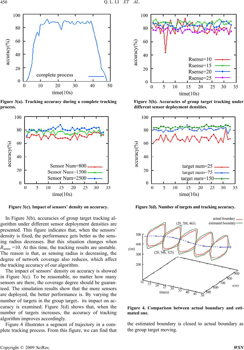

Q. L. LI ET AL. 450
Figure 3(a). Tracking accuracy during a complete tracking
process.
Figure 3(c). Impact of sensors’ density on accuracy.
In Figure 3(b), accuracies of group target tracking al-
gorithm under different sensor deployment densities are
presented. This figure indicates that, when the sensors’
density is fixed, the performance gets better as the sens-
ing radius decreases. But this situation changes when
Rsense =10. At this time, the tracking results are unstable.
The reason is that, as sensing radius is decreasing, the
degree of network coverage also reduces, which affect
the tracking accuracy of our algorithm.
Ted
Figure 3(c). To be reasonable, no matter how many
se
we can find that
he impact of sensors’ density on accuracy is show
in
nsors are there, the coverage degree should be guaran-
teed. The simulation results show that the more sensors
are deployed, the better performance is. By varying the
number of targets in the group target，its impact on ac-
curacy is examined. Figure 3(d) shows that, when the
number of targets increases, the accuracy of tracking
algorithm improves accordingly.
Figure 4 illustrates a segment of trajectory in a com-
plete tracking process. From this figure,
Figure 3(b). Accuracies of group target tracking under
different sensor deployment densities.
Figure 3(d). Number of targets and tracking accuracy.
Figure 4. Comparison between actual boundary and esti-
mated one.
the estimated boundary is closed to actual boundary as
the group target moving.

Q. L. LI ET AL. 451
5. Conclusions
The problem of group target tracking in wireless sensor
networks is fully investigated in this paper. To ach
the group target tracking goal, a flexible group targ
boundary detecting model is proposed. Moreover, utiliz-
ing a computing geometry conception—convex hull, a
novel divide-merge group target tracking algorith
proposed to solve this challenging problem. By an
ing the experimental results from simulations, the group
target tracking performance is evaluated. The results
show that the proposed algorithm is effective and effi-
cient.
n, J. C. Hou, and L. Sha, “Dynamic clusteri
G. Cao. “DCTC: Dynamic convo
, and S. Suri.
ao, and J. S. B. Mitchell,
CT: Collaborative event detection and tracking in
. Kesidis, “Dynamic
Computational geometry in C,”
and analysis of algorithms,” Addison-
sor
ieve
et
“Target tracking with binary proximity sensors: Funda-
mental limits, minimal descirptions, and algorithms,” In
Proceedings of ACM SenSys, 2006.
[6] X. Zhu, R. Sarkar, J. G
m is
alyz-
“Light-weight contour tracking in wireless sensor net-
works,” In Proceedings of IEEE INFOCOM, pp. 1849–
1857, 2008.
[7] K. P. Shih, S. S. Wang, P. H. Yang, and C. C. Chang,
“CollE
6. References
1] W. Che[ng for cluster structure for object detection and tracking in
wireless ad-hoc sensor networks,” IEEE International
Conference on Communications, Paris, FRANCE, June
20–24, 2004.
acoustic target tracking in wireless sensor networks,”
IEEE Transactions on Mobile Computing, Vol. 3, No. 3,
004. pp. 258–271, 2
2] W. Zhang and[y
[
tree-based collaboration for target tracking in sensor
networks,” IEEE Transactions on Wireless Communica-
tions, Vol. 3, No. 5, pp. 1689–1701, 2004.
[3] J. Aslam, Z. Butler, F. Constantin, V. Crespi, G. Cybenko,
and D. Rus, “Tracking a moving object with a binary sen-
sor network,” ACM Sensys’03, Los Angeles, California,
USA, pp. 150–161, 2003.
[4] J. Singh, U. Madhow, R. Kumar, S. Suri, and R. Cagley,
“Tracking multiple targets using binary proximity sen-
s,” In Proceedings of the 6th International Conference
on Information Processing In Sensor Networks, April
2007.
[5] N. Shrivastava, R. Mudumbai, U. Madhow
wireless heterogeneous sensor networks,” In Proceedings
of the 11th IEEE Symposium on Computers and Com-
munications (ISCC’06).
[8] X. Ji, H. Zha, John J. Metzner, and G
9] D. Cao, B. Jin, and J. Cao, “On group target tracking with
binary sensor networks,” In Proceedings of the 5th IEEE
International Conference on Mobile Ad Hoc and Sensor
System (MASS), pp. 334–339, 2008.
[10] O’ Rourke and Joseph, “
China Machine Press, 2005.
[11] T. H. Cormen, C. E. Leiseron, and R. L. Rivest. “Introduc-
tion to algorithms,” The MIT Press, pp. 947–956, 2002.
[12] R. C. T. Lee, S. S. Tseng, and R. C. Chang, “Introduction
to the design
Wesley, Chapter 12.6, 2002.

Q. L. LI ET AL. 452
Appendix
Dynamic approximation convex hull algorithm:
Input: A sequence of points with operators
, and the number
m of pairs of parallel lines being used.
Output: A sequence of approximate convex hulls
where is covering the reserve
here
Initialization: Construct m pairs of parallel lines with
I.
112 2
(,), (,),p operatorpoperator
12
,,aa,
points
i
a
,
l
p
, w
d
12
,,ppli.
slopes 0,tan(/),tan(2/), ,mm

 tan((1) /)mm  respec-
ti
f
vely antersect at the
ir
with ope
rs of par-
IF de
, Stop;
d locate all lines so that th
rator is1
(, )p insert .
ey all in
st input point1
p. Set i=1, i.e. the current input point
. IF (p is between each of the m paiStep 1i
allel lines)
(operator= lete) delete the point Pi,
1ll
ELSE insert the point Pi,1ll, Stop;
ELSE
IF (operator=delete) delete the point Pi,
1ll;
ELSE insert the point Pi, 1ll,'i
p
p

;
Step 2. Move e the linnearest to point, without
g
Step 3. Con
nectspect
in the clockwise fashion and denote this ap-
proximate convex hull as
Step 4. If no other point will be input, then stop; oth-
erwise, set i=i+1 and receive the next input
point as Pi. Go to Step 1.
raham-Scan(Q) // Algorithm which will be
Step 1.let
'p
changin its slope, to touch'pand associate
'pwith this line.
struct an approximate convex hull by con-
ing the 2m points with reto each line
j
a.
II. G
run on the sink
0
p
be the point in Q with the minimum
y
a
-coordinate, or the leftmost such point in case of
tie;
Step 2. let 12 ,,,
m
p
ppbe the remaining points in Q,
orted by polar angle in counterclockwise order
round 0
s
a
p
(if more than one point has the same
angle, remove all but the one that is farthest from
0
p
);
tep 3. PUSH(S0
p
,S);
Step 4. PUSH(1
p
,S);
5. PUSH(2
Step
p
,S);
Step 6. for(i=3, i<=m, i++)
ile(the angle
Step 8. POS(S
Step
Step 10turn S;
Step 7. {whformed by points
NEXT-TO-TOP(S), TOP(S), and Pi makes a
nonleft turn)
);
9. PUSH(Pi, S); }
. re