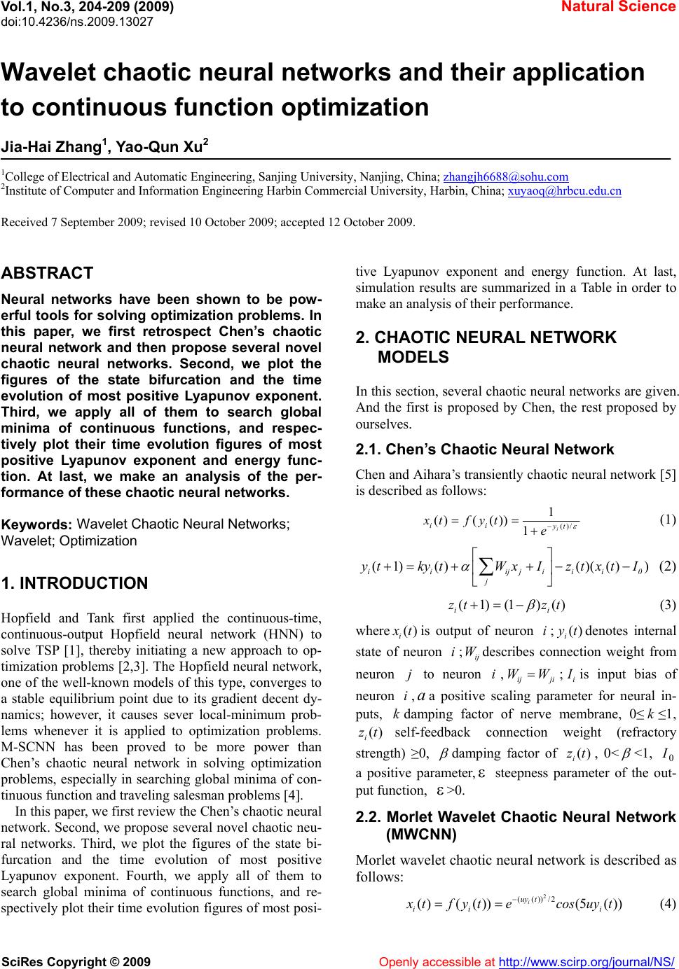Vol.1, No.3, 204-209 (2009)
doi:10.4236/ns.2009.13027
SciRes Copyright © 2009 Openly accessible at http://www.scirp.org/journal/NS/
Natural Science
Wavelet chaotic neural networks and their application
to continuous function optimization
Jia-Hai Zhang1, Yao-Qun Xu2
1College of Electrical and Automatic Engineering, Sanjing University, Nanjing, China;
2Institute of Computer and Information Engineering Harbin Commercial University, Harbin, China;
Received 7 September 2009; revised 10 October 2009; accepted 12 October 2009.
ABSTRACT
Neural networks have been shown to be pow-
erful tools for solving optimization problems. In
this paper, we first retrospect Chen’s chaotic
neural network and then propose several novel
chaotic neural networks. Second, we plot the
figures of the state bifurcation and the time
evolution of most positive Lyapunov exponent.
Third, we apply all of them to search global
minima of continuous functions, and respec-
tively plot their time evolution figures of most
positive Lyapunov exponent and energy func-
tion. At last, we make an analysis of the per-
formance of these chaotic neural networks.
Keywords: Wavelet Chaotic Neural Networks;
Wavelet; Optimization
1. INTRODUCTION
Hopfield and Tank first applied the continuous-time,
continuous-output Hopfield neural network (HNN) to
solve TSP [1], thereby initiating a new approach to op-
timization problems [2,3]. The Hopfield neural network,
one of the well-known models of this type, converges to
a stable equilibrium point due to its gradient decent dy-
namics; however, it causes sever local-minimum prob-
lems whenever it is applied to optimization problems.
M-SCNN has been proved to be more power than
Chen’s chaotic neural network in solving optimization
problems, especially in searching global minima of con-
tinuous function and traveling salesman problems [4].
In this paper, we first review the Chen’s chaotic neural
network. Second, we propose several novel chaotic neu-
ral networks. Third, we plot the figures of the state bi-
furcation and the time evolution of most positive
Lyapunov exponent. Fourth, we apply all of them to
search global minima of continuous functions, and re-
spectively plot their time evolution figures of most posi-
tive Lyapunov exponent and energy function. At last,
simulation results are summarized in a Table in order to
make an analysis of their performance.
2. CHAOTIC NEURAL NETWORK
MODELS
In this section, several chaotic neural networks are given.
And the first is proposed by Chen, the rest proposed by
ourselves.
2.1. Chen’s Chaotic Neural Network
Chen and Aihara’s transiently chaotic neural network [5]
is described as follows:
()/
1
()( ())1i
ii yt
xt fyte



 (1)
(1)()()(() )
ii ijjiii
j
ytkytWxIzt xtI 

 


0
i
(2)
(1)(1 )()
i
zt zt


 (3)
where ()
i
x
t
j
is output of neuron ;denotes internal
state of neuron ;Wdescribes connection weight from
neuron to neuron , ;
i
ji
WW
()
i
yt
i
iij
iij 
I
is input bias of
neuron ,aa positive scaling parameter for neural in-
puts, damping factor of nerve membrane, 0≤≤1,
self-feedback connection weight (refractory
strength) ≥0,
i
k k
()
i
zt

damping factor of , 0<()
i
zt

<1,
a positive parameter,
0
I

steepness parameter of the out-
put function,

>0.
2.2. Morlet Wavelet Chaotic Neural Network
(MWCNN)
Morlet wavelet chaotic neural network is described as
follows:
2
(())/2
()( ())(5())
i
uy t
ii i
x
tfyt ecosuyt

 (4)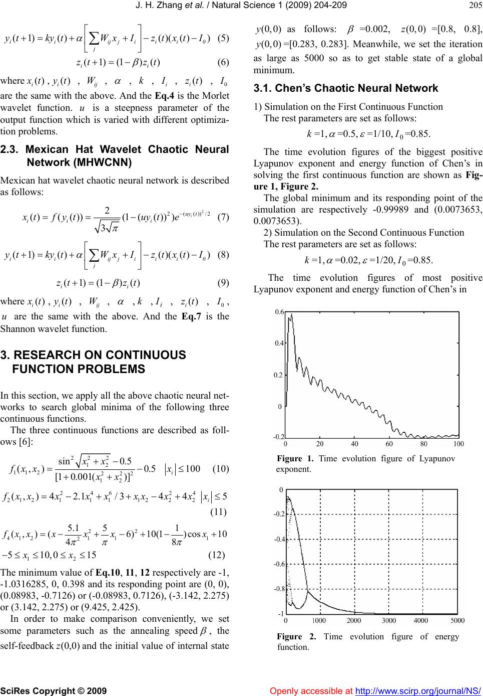

J. H. Zhang et al. / Natural Science 1 (2009) 204-209
SciRes Copyright © 2009 Openly accessible at http://www.scirp.org/journal/NS/
205
(1)()()(() )
ii ijjiii
j
ytkytWxIzt xtI 

 


0
i
(5)
(1)(1 )()
i
zt zt

 (6)
where ()
i
x
t, , , ()
i
yt ij W

, , ki
I
, , ()
i
zt 0
I
are the same with the above. And the Eq.4 is the Morlet
wavelet function. is a steepness parameter of the
output function which is varied with different optimiza-
tion problems.
u
2.3. Mexican Hat Wavelet Chaotic Neural
Network (MHWCNN)
Mexican hat wavelet chaotic neural network is described
as follows:
2
(())/2 2
2
( )(( ))(1(( )))
3
i
uy t
iii
xtfytuyt e


  (7)
(1)()()(() )
ii ijjiii
j
ytkytWxIzt xtI 

 


0
i
(8)
(1)(1)()
i
zt zt

 (9)
where ()
i
x
t, , , ()
i
yt ij W

,k , , ,
i
I()
i
zt 0
I
,
are the same with the above. And the Eq.7 is the
Shannon wavelet function.
u
3. RESEARCH ON CONTINUOUS
FUNCTION PROBLEMS
In this section, we apply all the above chaotic neural net-
works to search global minima of the following three
continuous functions.
The three continuous functions are described as foll-
ows [6]:
22 2
12
11 2222
12
sin 0.5
(, )0.5
[1 0.001()]
xx
fxx xx


 100
i
x (10)
2462
21211 11222
(, ) 42.1/344
4
f
xxxx xxxxx 5
i
x

(11)
22
4121 11
2
5.1 51
(,)(6)10(1) cos10
8 4
fxx xxxx
 
 
12
510,0 15xx  (12)
The minimum value of Eq.10, 11, 12 respectively are -1,
-1.0316285, 0, 0.398 and its responding point are (0, 0),
(0.08983, -0.7126) or (-0.08983, 0.7126), (-3.142, 2.275)
or (3.142, 2.275) or (9.425, 2.425).
In order to make comparison conveniently, we set
some parameters such as the annealing speed

, the
self-feedback and the initial value of internal state
as follows:
)0,0(z
(0,0)y

=0.002, =[0.8, 0.8],
=[0.283, 0.283]. Meanwhile, we set the iteration
as large as 5000 so as to get stable state of a global
minimum.
(0,0)z
(0,0)y
3.1. Chen’s Chaotic Neural Network
1) Simulation on the First Continuous Function
The rest parameters are set as follows:
k=1,

=0.5,

=1/10, =0.85.
0
I
The time evolution figures of the biggest positive
Lyapunov exponent and energy function of Chen’s in
solving the first continuous function are shown as Fig-
ure 1, Figure 2.
The global minimum and its responding point of the
simulation are respectively -0.99989 and (0.0073653,
0.0073653).
2) Simulation on the Second Continuous Function
The rest parameters are set as follows:
k=1,

=0.02,

=1/20, =0.85.
0
I
The time evolution figures of most positive
Lyapunov exponent and energy function of Chen’s in
Figure 1. Time evolution figure of Lyapunov
exponent.
Figure 2. Time evolution figure of energy
function.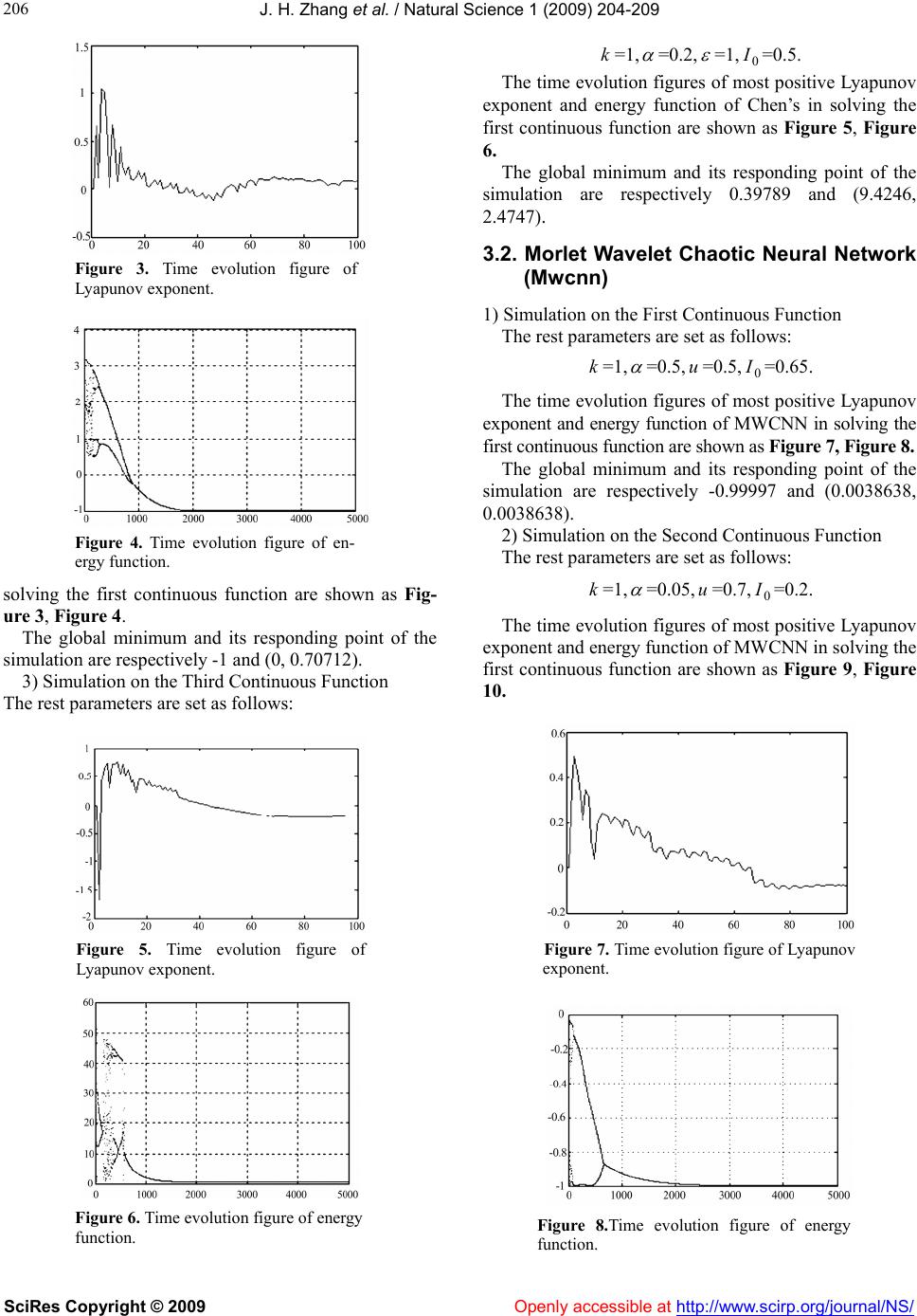

J. H. Zhang et al. / Natural Science 1 (2009) 204-209
SciRes Copyright © 2009 Openly accessible at http://www.scirp.org/journal/NS/
206
Figure 3. Time evolution figure of
Lyapunov exponent.
Figure 4. Time evolution figure of en-
ergy function.
solving the first continuous function are shown as Fig-
ure 3, Figure 4.
The global minimum and its responding point of the
simulation are respectively -1 and (0, 0.70712).
3) Simulation on the Third Continuous Function
The rest parameters are set as follows:
Figure 5. Time evolution figure of
Lyapunov exponent.
Figure 6. Time evolution figure of energy
function.
k=1,

=0.2,

=1, =0.5.
0
I
The time evolution figures of most positive Lyapunov
exponent and energy function of Chen’s in solving the
first continuous function are shown as Figure 5, Figure
6.
The global minimum and its responding point of the
simulation are respectively 0.39789 and (9.4246,
2.4747).
3.2. Morlet Wavelet Chaotic Neural Network
(Mwcnn)
1) Simulation on the First Continuous Function
The rest parameters are set as follows:
k=1,

=0.5, u=0.5, =0.65.
0
I
The time evolution figures of most positive Lyapunov
exponent and energy function of MWCNN in solving the
first continuous function are shown as Figure 7, Figure 8.
The global minimum and its responding point of the
simulation are respectively -0.99997 and (0.0038638,
0.0038638).
2) Simulation on the Second Continuous Function
The rest parameters are set as follows:
k=1,

=0.05, u=0.7, =0.2.
0
I
The time evolution figures of most positive Lyapunov
exponent and energy function of MWCNN in solving the
first continuous function are shown as Figure 9, Figure
10.
Figure 7. Time evolution figure of Lyapunov
exponent.
Figure 8.Time evolution figure of energy
function.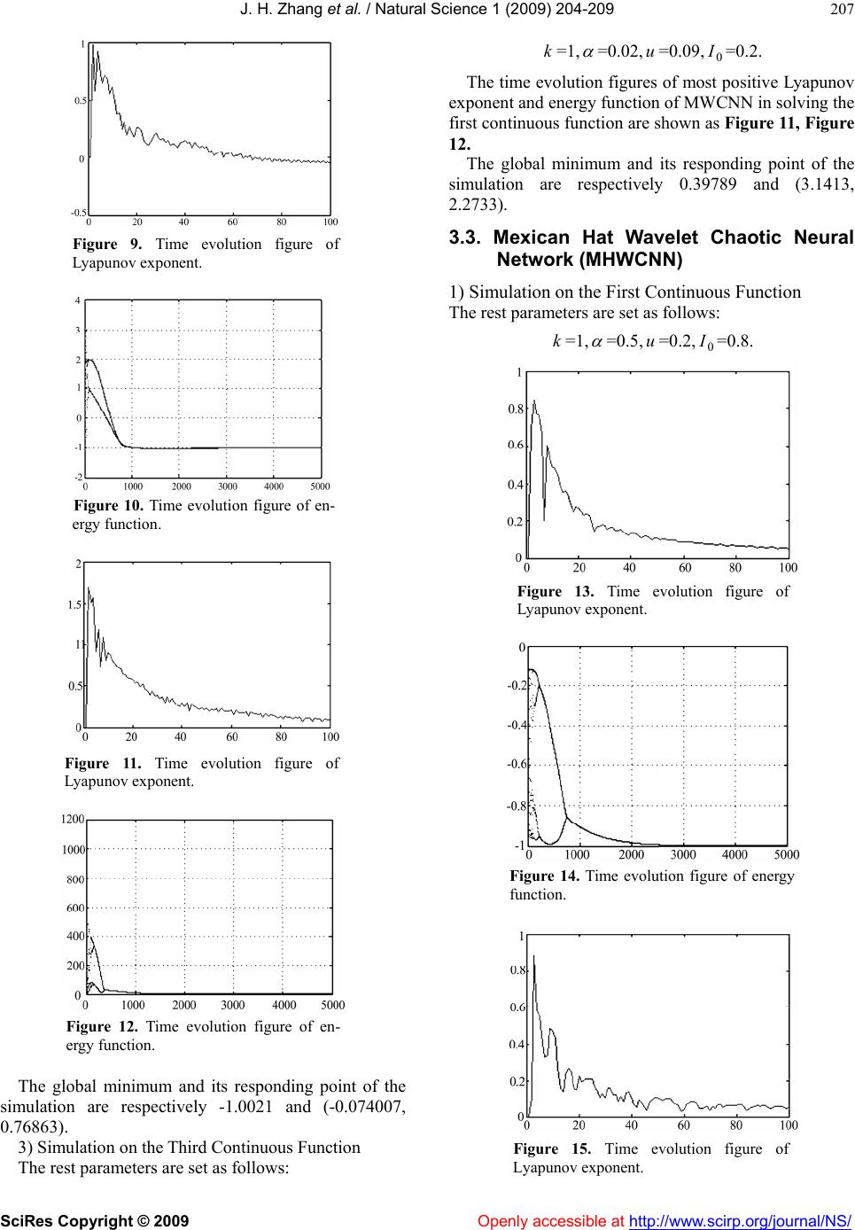

J. H. Zhang et al. / Natural Science 1 (2009) 204-209
SciRes Copyright © 2009 Openly accessible at http://www.scirp.org/journal/NS/
207
Figure 9. Time evolution figure of
Lyapunov exponent.
Figure 10. Time evolution figure of en-
ergy function.
Figure 11. Time evolution figure of
Lyapunov exponent.
Figure 12. Time evolution figure of en-
ergy function.
The global minimum and its responding point of the
simulation are respectively -1.0021 and (-0.074007,
0.76863).
3) Simulation on the Third Continuous Function
The rest parameters are set as follows:
k=1,

=0.02, u=0.09, =0.2.
0
I
The time evolution figures of most positive Lyapunov
exponent and energy function of MWCNN in solving the
first continuous function are shown as Figure 11, Figure
12.
The global minimum and its responding point of the
simulation are respectively 0.39789 and (3.1413,
2.2733).
3.3. Mexican Hat Wavelet Chaotic Neural
Network (MHWCNN)
1) Simulation on the First Continuous Function
The rest parameters are set as follows:
k=1,

=0.5, =0.2,=0.8. u0 I
Figure 13. Time evolution figure of
Lyapunov exponent.
Figure 14. Time evolution figure of energy
function.
Figure 15. Time evolution figure of
Lyapunov exponent.

J. H. Zhang et al. / Natural Science 1 (2009) 204-209
SciRes Copyright © 2009 http://www.scirp.org/journal/NS/
208
Table 1. the simulation results of the chaotic neural networks.
The time evolution figures of most positive Lyapunov
exponent and energy function of MHWCNN in solving
Fu
n
Model
GM/ER
Chen’s MWCNN MHWCNN
TGM -1 -1 -1
PGM -0.99989 -0.99997 -0.99996
1
f
ER 0.00011 0.00003 0.00004
TGM -1.0316285 -1.0316285 -1.0316285
PGM -1 -1.00021 -1.0316
2
f
ER 0.0316285 0.031418
5
0.0000285
TGM 0.398 0.398 0.398
PGM 0.3789 0.3789 0.3789
4
f
ER 0.0191 0.0191 0.0191
AVEAVER 0.01270962 0.01263712 0.00479212
the first continuous function are shown as Figure 13,
Figure 14.
The global minimum and its responding point of the
simulation are respectively -0.99996 and (0.0043259,
0.0043259).
2) Simulation on the Second Continuous Function
The rest parameters are set as follows:
k=1,

=0.05, u=2.8, =0.05.
0
I
The time evolution figures of most positive Lyapunov
exponent and energy function of MHWCNN in solving
the first continuous function are shown as Figure 15,
Figure 16.
The global minimum and its responding point of the
simulation are respectively -1.0316 and (-0.089825,
0.71263).
3) Simulation on the Third Continuous Function.
The rest parameters are set as follows:
k=1,

=0.05, =0.3, =0.2. u0 I
The time evolution figures of most positive Lyapunov
exponent and energy function of MHWCNN in solving
the first continuous function are shown as Figure 17,
Figure 18.
Figure 16. Time evolution figure of en-
ergy function.
The global minimum and its responding point of the
simulation are respectively 0.39789 and (3.1415,
2.2743).
4. ANALYSIS OF THE SIMULATION
RESULTS
Simulation results are summarized in Table 1. The col-
umns “GM/ER”, “TGM”, “PGM” and “AVER” repre-
sent, respectively, global minimum/error rate; theoretical
global minimum; practical global minimum; average
error.
Figure 17. Time evolution figure of
Lyapunov exponent.
Seen from the Table 1, we can conclude that the
wavelet chaotic neural networks are superior to Chen’s
in AVER
5. CONCLUSION
We have introduced Chen’s and wavelet chaotic neural
networks. We make an analysis of them in solving con-
tinuous function optimization problems, and find out that
wavelet chaotic neural networks are superior to Chen’s
in general.
Figure 18. Time evolution figure of en-
ergy function.
Openly accessible at

J. H. Zhang et al. / Natural Science 1 (2009) 204-209
SciRes Copyright © 2009 Openly accessible at http://www.scirp.org/journal/NS/
209
REFERENCES
[1] J. J. Hopfield and D. W. Tank, (1985) Neural com-
putation of decision in optimization problems. Biol.
Cybern., 52, 141-152.
[2] J. Hopfield, (1982) Neural networks and physical systems
with emergent collective computa-tional abilities. In:
Proc Natl Acad Sci, 79, 2554-2558.
[3] J. Hopfield, (1984) Neural networks and physical systems
with emergent collective computational abilities. 81, Proc.
Natl. Acad. Sci., 3088-3092.
[4] Y. Q. Xu, M. Sun, and G. R. Duan, (2006) Wavelet
chaotic neural networks and their application to optimi-
zation problems. Lecture Notes in Computer Science.
[5] L. P. Wang and F. Y. Tian, (2000) Noisy chaotic neural
networks for solving combinatorial optimization pro-
blems. International Joint Conference on Neural Net-
works. Italy, IEEE, 37-40.
[6] L. Chen and K. Aihara, (1995) Chaotic simulated
annealing by a neural network model with transient chaos.
Neural Networks., 8, 915-930.
[7] L. Wang, (2001) Intelligence optimization algorithm and
its application. Press of TUP.
[8] C. Q. Xie, C. He, and H. W. Zhu, (2002) Improved noisy
chaotic neural networks for solving combinational opti-
mization problems. Journal of Shanghai Jiaotong univer-
sity, 36, 351-354.
[9] Y. Q. Xu and M. Sun, (2006) Gauss-morlet-sigmoid cha-
otic neural networks. ICIC, LNCS.