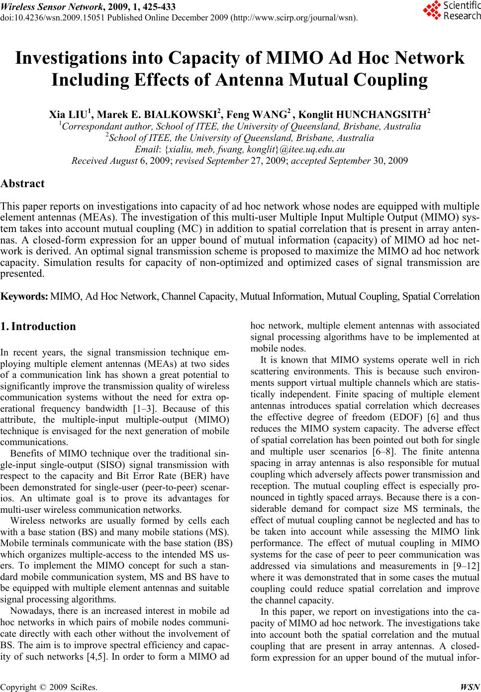Wireless Sensor Network, 2009, 1, 425-433
doi:10.4236/wsn.2009.15051 Published Online December 2009 (http://www.scirp.org/journal/wsn).
Investigations into Capacity of MIMO Ad Hoc Network
Including Effects of Antenna Mutual Coupling
Xia LIU1, Marek E. BIALKOWSKI2, Feng WANG2 , Konglit HUNCHANGSITH2
1Correspondant author, School of ITEE, the University of Queensland, Brisbane, Australia
2School of ITEE, the University of Queensland, Brisbane, Australia
Received August 6, 2009; revised September 27, 2009; accepted September 30, 2009
Abstract
This paper reports on investigations into capacity of ad hoc network whose nodes are equipped with multiple
element antennas (MEAs). The investigation of this multi-user Multiple Input Multiple Output (MIMO) sys-
tem takes into account mutual coupling (MC) in addition to spatial correlation that is present in array anten-
nas. A closed-form expression for an upper bound of mutual information (capacity) of MIMO ad hoc net-
work is derived. An optimal signal transmission scheme is proposed to maximize the MIMO ad hoc network
capacity. Simulation results for capacity of non-optimized and optimized cases of signal transmission are
presented.
Keywords: MIMO, Ad Hoc Network, Channel Capacity, Mutual Information, Mutual Coupling, Spatial Correlation
1. Introduction
In recent years, the signal transmission technique em-
ploying multiple element antennas (MEAs) at two sides
of a communication link has shown a great potential to
significantly improve the transmission quality of wireless
communication systems without the need for extra op-
erational frequency bandwidth [1–3]. Because of this
attribute, the multiple-input multiple-output (MIMO)
technique is envisaged for the next generation of mobile
communications.
Benefits of MIMO technique over the traditional sin-
gle-input single-output (SISO) signal transmission with
respect to the capacity and Bit Error Rate (BER) have
been demonstrated for single-user (peer-to-peer) scenar-
ios. An ultimate goal is to prove its advantages for
multi-user wireless communication networks.
Wireless networks are usually formed by cells each
with a base station (BS) and many mobile stations (MS).
Mobile terminals communicate with the base station (BS)
which organizes multiple-access to the intended MS us-
ers. To implement the MIMO concept for such a stan-
dard mobile communication system, MS and BS have to
be equipped with multiple element antennas and suitable
signal processing algorithms.
Nowadays, there is an increased interest in mobile ad
hoc networks in which pairs of mobile nodes communi-
cate directly with each other without the involvement of
BS. The aim is to improve spectral efficiency and capac-
ity of such networks [4,5]. In order to form a MIMO ad
hoc network, multiple element antennas with associated
signal processing algorithms have to be implemented at
mobile nodes.
It is known that MIMO systems operate well in rich
scattering environments. This is because such environ-
ments support virtual multiple channels which are statis-
tically independent. Finite spacing of multiple element
antennas introduces spatial correlation which decreases
the effective degree of freedom (EDOF) [6] and thus
reduces the MIMO system capacity. The adverse effect
of spatial correlation has been pointed out both for single
and multiple user scenarios [6–8]. The finite antenna
spacing in array antennas is also responsible for mutual
coupling which adversely affects power transmission and
reception. The mutual coupling effect is especially pro-
nounced in tightly spaced arrays. Because there is a con-
siderable demand for compact size MS terminals, the
effect of mutual coupling cannot be neglected and has to
be taken into account while assessing the MIMO link
performance. The effect of mutual coupling in MIMO
systems for the case of peer to peer communication was
addressed via simulations and measurements in [9–12]
where it was demonstrated that in some cases the mutual
coupling could reduce spatial correlation and improve
the channel capacity.
In this paper, we report on investigations into the ca-
pacity of MIMO ad hoc network. The investigations take
into account both the spatial correlation and the mutual
coupling that are present in array antennas. A closed-
form expression for an upper bound of the mutual infor-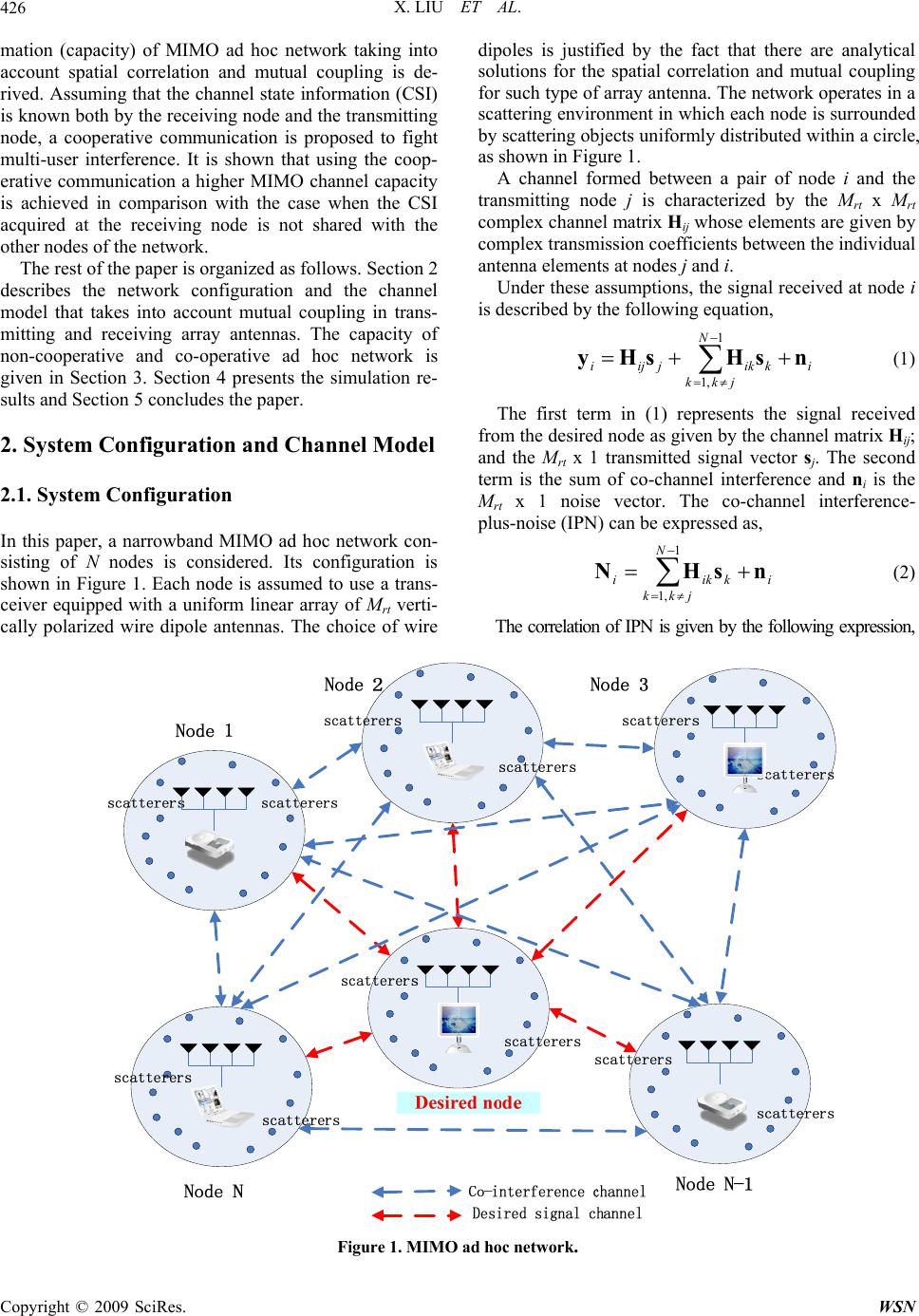

X. LIU ET AL. 426
mation (capacity) of MIMO ad hoc network taking into
account spatial correlation and mutual coupling is de-
rived. Assuming that the channel state information (CSI)
is known both by the receiving node and the transmitting
node, a cooperative communication is proposed to fight
multi-user interference. It is shown that using the coop-
erative communication a higher MIMO channel capacity
is achieved in comparison with the case when the CSI
acquired at the receiving node is not shared with the
other nodes of the network.
The rest of the paper is organized as follows. Section 2
describes the network configuration and the channel
model that takes into account mutual coupling in trans-
mitting and receiving array antennas. The capacity of
non-cooperative and co-operative ad hoc network is
given in Section 3. Section 4 presents the simulation re-
sults and Section 5 concludes the paper.
2. System Configuration and Channel Model
2.1. System Configuration
In this paper, a narrowband MIMO ad hoc network con-
sisting of N nodes is considered. Its configuration is
shown in Figure 1. Each node is assumed to use a trans-
ceiver equipped with a uniform linear array of Mrt verti-
cally polarized wire dipole antennas. The choice of wire
dipoles is justified by the fact that there are analytical
solutions for the spatial correlation and mutual coupling
for such type of array antenna. The network operates in a
scattering environment in which each node is surrounded
by scattering objects uniformly distributed within a circle,
as shown in Figure 1.
A channel formed between a pair of node i and the
transmitting node j is characterized by the Mrt x Mrt
complex channel matrix Hij whose elements are given by
complex transmission coefficients between the individual
antenna elements at nodes j and i.
Under these assumptions, the signal received at node i
is described by the following equation,



 1
,1
N
jkk
ikikjiji nsHsHy (1)
The first term in (1) represents the signal received
from the desired node as given by the channel matrix Hij;
and the Mrt x 1 transmitted signal vector sj. The second
term is the sum of co-channel interference and ni is the
Mrt x 1 noise vector. The co-channel interference-
plus-noise (IPN) can be expressed as,



 1
,1
N
jkk
ikiki nsHN (2)
The correlation of IPN is given by the following expression,
Figure 1. MIMO ad ho c n etwork .

X. LIU ET AL. 427
M
1
2
1,
{}
irt
N
HH
Nii ikkikn
kkj
RENNQ I 


 
HH (3)
where Qk= E{sksk
H} is the data covariance matrix repre-
senting the signal transmission scheme from the k-th
inference node to node i. E{} denotes the statistical ex-
pectation.
For the case of non-optimized ad hoc network, only
receivers have the knowledge of CSI. In such a case, the
best strategy for the nodes is to transmit equal power
over the individual transmitting antenna elements. In this
case, the Qik of the k-th interference node can be ex-
pressed as:
1
12
1
,
:, ...
k
ik
t
N
I
k
k
p
QI
N
k
s
ubjectto Ppppp





(4)
where pk is the transmit power from node k and PI is the
total transmitted power of all interferences.
By using (4), Equation (3) can be rewritten as:
1
2
1,
1
i
N
H I
Nikik
kkj
P
R
N




HH rt
nM
I
N
(5)
The correlation of received signal at node i that is
transmitted from the desired node is obtained as:
{} i
yH H
iiiijjij
REyyQ R HH (6)
in which Qj= E{sjsj
H} is the data covariance matrix rep-
resenting the signal transmission scheme from node j to
node I, which is also the mutual information for the
channel formed between the desired node j and node i.
tr{Qj}=Pj and Pj is the total transmitted signal power
from the desired node.
The capacity of the system can be improved by opti-
mizing the signal transmission scheme. The optimization
process requires the knowledge of CSI by transmitters
which is usually obtained by a feedback loop from re-
ceivers. In this case, the new data correlation matrix,
subject to constraint of total transmitted power tr{Qj}=Pj,
has to be worked out.
2.2. Channel Model Neglecting Mutual Coupling
In the undertaken investigations, a narrow-band flat
block-fading MIMO channel is assumed between the
network nodes. For each pair of nodes, the channel ma-
trix (H) can be used to describe the channel properties.
Its entries depend on the signal propagation environment
and properties of the antenna arrays used at the two sides
of communication link.
In the initial stage, the Kronecker representation of
channel [13,14] neglecting the effects of mutual coupling
is assumed. In this representation, the transmitter and
receiver correlations are separable and the channel ma-
trix H (for brevity the subscripts are dropped here) is
represented as:
1/2 1/2
R
HT
RGRH (7)
where GH is the matrix including identical independent
distributed (i.i.d) Gaussian entries with zero mean and
unit variance, and RR
}
)
and RT are the spatial correlation
matrices at the receiver and transmitter, respectively. The
channel correlation is expressed as,
{
H
H
REHH (8)
Because each node includes vertically polarized wire
dipole antennas and the scattering environment is repre-
sented by circles of uniformly distributed scattering ob-
jects surrounding nodes as shown in Fig.1, the spatial
correlation matrix elements can be obtained using the
Clark’s model as given by.
()
,0,
(
RT
lm lm
Jd   (9)
where J0 stands for the zero-order Bessel function, κ is a
wave number and dlm is the distance between elements l
and m of the uniform array antenna.
The correlation matrices RT and RR can be generated
using (9) as,
() ()
1,1 1,
()
() ()
,,
rt
rtrt rt
RT RT
M
RT
RT RT
Mj MM
R














 

(10)
Having defined RT and RR
I
T
, the channel matrix for each
pair of nodes (H) can be calculated using Equation (7).
2.3. Channel Model Including Mutual Coupling
The mutual coupling in an array of collinear side-by-side
wire dipoles can be modeled using the theory described
in [16]. Assuming the array is formed by Mrt wire dipoles,
the mutual matrix can be calculated using the following
expression
1
(ΖΖ)( )
rt
AT TM

 ZC (11)
where Z is the impedance matrix, ZA is the element input
impedance in isolation, e.g. when the wire dipole is λ/2,
its value is ZA=73+j42.5[Ω]; ZT is impedance of the re-
ceiver chosen as the complex conjugate of ZA to obtain
the impedance match for best power transfer.
The impedance matrix Z is given by
12 1
21 2
12
rt
rt
rt rt
AT M
AT M
MM A
ZZ ZZ
ZZZ Z
Z
ZZ

Z
















Z=




(12)

X. LIU ET AL. 428
n
Note that this expression provides the circuit repre-
sentation for mutual coupling in array antennas. It is
valid for single mode antennas. Wire dipoles fall into this
category.
For the side-by-side configuration of dipoles having
length l equal to 0.5λ, the expressions for {Zmn} can be
adapted from [16,17] and are rewritten here as,
012
012
30[0.5772 ln(2)(2)]
[30 (2)],
30[2() () ()]
[30(2()( )())],
i
i
mn
iii
iii
lC l
jS lmn
CuCuCu
jSuSuSum










Z= (13)
where κ is the wave number equal to 2π/λ,
0
22
1
22
2
,
(
()
h
h
h
ud
udl
udl






) l
l
(14)
dh is the horizontal distance between the two dipole
antenna elements. Ci(u) and Si(u) are the cosine and sine
integrals, respectively. They are given as,
0
()(cos()/ )
()(sin()/ )
u
i
i
Cux xdx
Sux xdx





 (15)
The expression for the coupling matrix (11) can be
used both at the transmitting and receiving nodes to
modify the channel matrices and the correlation matrices.
When the mutual coupling is included, the channels ma-
trices H shown in (7) has to be modified to the new form
given by
'
R
T
CCHH (16)
where the mutual coupling matrices are calculated using
(11).
Similarly, the receiving and transmitting correlation
matrices are modified using
1
2
R
muR R
RCR (17)
1
2
TmuT T
RRC (18)
3. Capacity of MIMO Ad Hoc Network
3.1. Channel Capacity between Individual Nodes
Having derived the channel matrices between the indi-
vidual notes for the cases without and with mutual cou-
pling, the next step is to obtain the channel capacities.
The mutual information of the channel formed between
node i and the desired transmitting node j of MIMO
ad-hoc network can be obtained in a similar way as for
the case of a multi-access MIMO system [15] and is
given as:
,
,
,,
,
(; |)
(; |,,)
(|,, )(|,,, )
(|, ,) ()
ij kkj
ijkkjijik
ikkj ij ikikkjj ij ik
ikkj ij iki
Iys s
Iys s
hy shy ss
hy shN







HH
HH HH
HH
(19)
The upper bound for capacity can be obtained from
the following,
,
22
1
22
11
22
22
(; |)
{log det[()]log det()}
{log det()]}
{logdet( ()())]}
ii
I
rt
rti i
ij kkj
H
ij jijNN
H
Nijjij
M
n
jH
MNijNij
n
Iys s
EeQR eR
RQ
EI
Q
EIRR









HH
HH
HH
(20)
where σn
2 is the noise power.
When both the Kronecker representation (7) and the
mutual coupling (11) are included in the MIMO channel
model, the expression (20) for the upper bound of mutual
information of the channel formed between node i and
the desired transmitting node j of MIMO ad-hoc network
is modified to:
2
11
22
2
(; |)
{log det[
()(
rt
iij iij
ij ik
M
jjj jjH
NRmuHTmuNRmuHTmu
n
Iys s
EI
QRR GRRR GR



)]}
(21)
The correlation of IPN with mutual coupling is given
by (22),
1
2
1
()()
iikik
N
muikikikik H
I
NRmuHTmuRmuHTmu
i
P
RRGRRGR
N




rt
nM
I
(22)
The expression for the upper bound of mutual infor-
mation (21) is given for a specified signal transmission
scheme as described by the data covariance matrix Q
j=
E{sjsj
H}.
The mutual information can be maximized by opti-
mizing the signal transmission scheme subject to
tr{Qj}=Pj. As a a result, the capacity between the i-th
node and the desired transmitting node for the optimized
signal transmission scheme is given by
22 2
(/) /
11
22
2
max{log det[
()(
rt
jn jn
iijiij
iM
tr QP
jij ijij ijH
NRmu HTmuNRmu HTmu
n
CEI
QRR GRRR GR





)]}
(23)
3.2. Capacity of Non-Cooperative Network
The capacity of ad hoc network that uses the optimized
transmission scheme between individual nodes can be

X. LIU ET AL.429
written as the sum of individual optimized link capacities
Ci and therefore can be expressed as,
1
11
22
22
1
{log det[()()]}
rti iji ij
N
i
i
Njij ijijijH
MNRmu HTmuNRmu HTmu
in
CC
Q
EIRR GRRR GR








(24)
3.3. Capacity of Cooperative Network
The capacity of ad hoc network can be further improved
by assuming cooperation between individual nodes. To
accomplish this, first the desired transmitting node has to
have the knowledge of channel state information (CSI)
from all the remaining nodes of the network. This means
that all of the complex channel matrices Hij are perfectly
known to the transmitting nodes. In practice, the required
CSI is first acquired by receivers by using the training
sequences between the pairs of nodes and by applying
the channel estimation at receiver. Next, it is passed to
transmitters using the feedback loops between the re-
ceivers and the transmitters.
To make the ad hoc network fully cooperative another
assumption is made that each of the N nodes not only
feeds information about the channel properties but also
provides the information about the interference to the
desired transmitting node. Under these conditions, the
desired transmitting node applies N different signal
transmission schemes to N receiving nodes to maximize
the mutual information (channel capacity) to each node.
This strategy leads to optimization of the overall capacity
of ad hoc network.
In order to obtain the capacity of the cooperative net-
work, first we introduce the combined channel correla-
tion in terms of channel Hij as,
1
1
()(
I
iji ij
H
combijN ij
ij ijHij ij)
R
mu HTmuNRmu HTmu
RR
RGR RRGR




HH (25)
In order to optimize the channel capacity between
node i and the desired transmitting node j a water-filling
algorithm can be applied. Using this algorithm, the opti-
mized channel capacity can be expressed as:
22
1
log (1)
rt ij
M
opt ij m
i
mn
p
Cm




 (26)
in which pm
ij is the optimal transmitted power from the
desired transmitting node j to node i, which is the subject
to the condition
1
rt
M
ij
j
m
m
Pp

 (27)
λm
ij is the m-th eigenvalue of combined channel corre-
lation Rcomb given by (25).
The optimal transmitted power at the m-th antenna is
obtained using the following equation,
1
1
()
:
rt
ijij ij
m
M
ij
mi
m
p
j
s
ubject topP






(28)
in which (x)+=max(0, x) and μ is chosen to obey the
power constraint. The capacity of the cooperative ad hoc
network with the optimized signal transmission scheme
is given as,
22
111
log (1)
rt ij
M
NN
opt optij m
im
iimn
p
CC



 
 (29)
4. Simulation Results
In this section, computer simulations are performed to
investigate the effects of spatial correlation and mutual
coupling on capacity of ad hoc network. In the under-
taken simulations, each node of ad hoc network is as-
sumed to be equipped with a 4-element uniform array
antenna. The elements are assumed to be wire dipoles
having length of 0.5λ, where λ is the carrier wavelength.
The transmit/receive spatial correlation matrices for each
pair of nodes are obtained using Equations (9) and (10)
as presented in Subsection 2.2. The mutual coupling ma-
trices are obtained from expressions (17) and (18) as
given in Subsection 4.3.
Figure 2 presents the ad hoc network capacity in a
2-dimentional (2D) manner. The X and Y axis represent
the capacity as an empirical distribution function (EDF),
which is a cumulative probability 1/M at each of the M
numbers in a sample,
1
1
( )(),1,...,
M
i
Mi
i
Xx
F
xIXxi
MM


 
M
(35)
46810 12 14
0
0.1
0.2
0.3
0.4
0.5
0.6
0.7
0.8
0.9
1
Capacity
Probability = F(Capacity)
Empirical Cumulative Distribution Function of System Capacity
dipole spacing d=0.2λ no MC
dipole spacing d=0.5λ no MC
dipole spacing d=0.2λ with MC
dipole spacing d=0.5λ with MC
i.i.d channel
Figure 2. The empirical distribution function (EDF) of ca-
pacity of single user vs multiple user MIMO system.

X. LIU ET AL. 430
where Xi is the i-th element in the sample and I(A) is the
indicator of event A. The X-axis represents the capacity
while Y-axis indicates probability.
It can be seen in Figure 2 that when the spatial corre-
lation exists, the capacity of ad hoc network is lower than
when an ideal independent identical distribution (i.i.d)
channel is assumed. This confirms the findings already
obtained for single-user and multi-access MIMO systems
reported in [8].
The presented results also show that when the dipole
antenna spacing is small and equal to 0.2λ, the capacity
with mutual coupling effect is larger compared to the one
when mutual coupling is neglected. When the spacing is
increased to 0.5λ the capacity curves, for with and with-
out mutual coupling effect, are getting very close to each
other. The gap between these curves is getting smaller.
The results obtained for the 4-element linear wire di-
pole arrays indicate that at the element spacing of 0.2λ,
mutual coupling decreases spatial correlation level and
improves capacity. When the spacing becomes larger, the
mutual coupling effect becomes less pronounced and
there is not much difference in capacity results when the
mutual coupling is neglected or taken into consideration.
Figure 3 presents the ad hoc network capacity in a
3-dimentional (3D) manner. The X and Y axes represent
the capacity as an empirical distribution function (EDF),
similarly as in Figure 2. In comparison with Figure 2, the
Z axis is added to indicate the antenna spacing between
the adjacent dipoles. There are two surfaces representing
the ad hoc network capacity. One surface represents the
case of antenna arrays without mutual coupling while the
other one stands for the case when the mutual coupling
effect is included in calculations. From the results pre-
sented in Figure 3, one can see that when the dipole
spacing is within 0.2λ to 0.4λ, at a fixed high probability,
the capacity of ad hoc network with mutual coupling
effect is higher than when mutual coupling is not taken
into account. The trend becomes opposite when the
spacing gets larger and is in the range of 0.4λ to 0.6λ. A
cross-point occurs at the spacing equal to 0.4λ. For the
element spacing of 0.6λ to 1λ, two surfaces overlap. The
observed trends indicate that when the spacing is small
(0.2λ to 0.4λ), the mutual coupling decreases spatial cor-
relation and improves capacity. When the spacing is in
the range of 0.4λ to 0.6λ, the mutual coupling increases
the spatial correlation and decreases capacity. When the
spacing exceeds 0.6λ, the mutual coupling weakly affects
capacity and thus can be neglected because two sets of
results without and with mutual coupling are almost
identical.
Figure 4 shows the results similar to those of Figure 3
but for the case of non-optimized and optimized signal
transmission schemes as given by expression (24) and
(29), respectively.
The results shown in Figure 4 reveal that signal trans-
mission optimization significantly improves ad hoc net-
work capacity for both cases when mutual coupling is
neglected or taken into account. The gap between the
two capacity surfaces, with and without mutual coupling,
is larger than for the non-optimized transmission scheme
presented in Figure 3.
The differences between the non-optimized (expression (24))
0.1
0.2
0.3
0.4
0.5
0.6
0.7
0.8
0.9
2
3
4
5
6
7
8
0
0.2
0.4
0.6
0.8
1
Anenna Spacing d/λ
Capacity
Probability
with MC
without MC
0.1
0.2
0.3
0.4
0.5
0.6
0.7
0.8
0.9
Figure 3. The empirical d is t ribu tion function (EDF) of capacity
vs Antenna spacing with and without mutual coupling (MC)

X. LIU ET AL.431
0.1
0.2
0.3
0.4
0.5
0.6
0.7
0.8
0.9
2
4
6
8
10
12
14
0
0.5
1
Antenna Spacing d/λ
Capacity
Probability
0.1
0.2
0.3
0.4
0.5
0.6
0.7
0.8
0.9
non-optimized without MC
optimized with MC
non-optimized without MC
optimized with MC
Figure 4. Non-optimized and optimized capacity vs Antenna spacing with and without mutual coupling (MC)
0
0.2
0.4
0.6
0.8
1
0
5
10
15
0
5
10
15
20
25
30
35
40
45
Antanna Spacing d/λ
Non-optimized vs optimized capacity without mutual coupling (MC)
SNR (dB)
Capacity
5
10
15
20
25
30
35
40
Optimized Capacity
Non-optimized Capacity
0
0.2
0.4
0.6
0.8
1
0
5
10
15
0
5
10
15
20
25
30
35
40
45
Antenna spcing d/λ
Non-optimzied vs optimzied capacity with mutual coupling (MC)
SNR (dB)
Capacity
5
10
15
20
25
30
35
40
Optimized Capacity
Non-optimized Capacity
A. Non-optimized vs optimized capacity without MC B. Non-optimized vs optimized capacity with MC
Figure 5. Non-optimized vs optimized ergodic capacity with and without mutual coupling.
and optimized (expression (29)) signal transmission
cases can also be investigated in terms of ergodic capac-
ity.
Figure 5 presents in the 3D manner the results for er-
godic capacity versus antenna spacing (from 0.1λ to 1λ)
and SNR (from 0 to 15dB) for non-optimized as given by
expression (29) and optimized as given by expression
(24) signal transmission schemes.
Figure 5A presents the results when the mutual cou-
pling effect is neglected, while Figure 5B shows the re-
sults when the mutual coupling effect is taken into ac-
count. One can see from the two Figures that irrespective
of including or neglecting mutual coupling, the capacity
for the optimized signal transmission scheme is higher
than for the non-optimized case.
Figure 6 is another representation of results shown in
Figure 5 when the signal transmission scheme is non-
optimized.
Figure 6A presents the capacity without mutual cou-
pling while Figure 6B presents the capacity when the
mutual coupling effect is taken into account. One can see
at spacing from 0.1λ to 0.4λ, that the capacity under mutual

X. LIU ET AL. 432
0.2
0.4
0.6
0.8
05 10 15
Spacing: 0.2
SNR: 14dB
Capacity: 30.37
Spacing: 0.4
SNR: 14dB
Capacity: 27.57
Spacing: 0.4
SNR: 13dB
Capacity: 24.59
SNR (dB)
A. Non-optimized capacity without mutual coupling (MC)
Antenna spacing d/λ
5
10
15
20
25
30
35
40
0.2
0.4
0.6
0.8
05 10 15
Spacing: 0.2
SNR: 14dB
Capacity: 31.61
Spacing: 0.4
SNR: 14dB
Capacity: 29.88
Spacing: 0.4
SNR: 13dB
Capacity: 26.38
SNR (dB)
B. Non-optimized capacity with mutual coupling (MC)
Antenna spacing d/λ
5
10
15
20
25
30
35
40
Spacing: 0.2λ
SNR: 14dB
Capacity: 30.37
Spacing: 0.4λ
SNR: 13dB
Capacity: 24.59
Spacing: 0.4λ
SNR: 14dB
Capacity: 27.57
Spacing: 0.2λ
SNR: 14dB
Capacity: 31.61
Spacing: 0.4λ
SNR: 13dB
Capacity: 26.38
Spacing: 0.4λ
SNR: 14dB
Capacity: 29.88
Figure 6. 2-D view of non-optimized ergodic capacity with-
out (A) and with (B) mutual coupling 2-D view.
0.2
0.4
0.6
0.8
05 10 15
Spacing: 0.2
SNR: 14dB
Capacity: 36.34
Spacing: 0.4
SNR: 14dB
Capacity: 34.55
Spacing: 0.4
SNR: 13dB
Capacity: 31.11
SNR (dB)
A. Optimized capacity without mutual coupling (MC)
Antenna Spacing d/λ
5
10
15
20
25
30
35
40
0.2
0.4
0.6
0.8
05 10 15
Spacing: 0.2
SNR: 14dB
Capacity: 36.99
Spacing: 0.4
SNR: 14dB
Capacity: 35.93
Spacing: 0.4
SNR: 13dB
Capacity: 32.44
SNR (dB)
B. Optimized capacity with mutual coupling (MC)
Antenna spacing d/λ
5
10
15
20
25
30
35
40
Spacing: 0.2λ
SNR: 14dB
Capacity: 36.34
Spacing: 0.4λ
SNR: 13dB
Capacity: 31.11
Spacing: 0.4λ
SNR: 14dB
Capacity: 34.55
Spacing: 0.2λ
SNR: 14dB
Capacity: 36.99
Spacing: 0.4λ
SNR: 13dB
Capacity: 32.44
Spacing: 0.4λ
SNR: 14dB
Capacity: 35.93
Figure 7. Optimized ergodic capacity without (A) and with
(B) mutual coupling (MC) 2-D view.
coupling effect is higher than the one with no mutual
coupling consideration. This property is more apparent at
higher values of SNR.
Similarly, Figure 7 provides another representation of
results shown in Figure 5 for the case when the signal
transmission scheme is optimized. Figure 7A presents
the capacity when mutual coupling is neglected while
Figure 7B presents the capacity with the mutual coupling
effect taken into account. One can see that at spacing
between 0.1λ to 0.4λ the capacity under mutual coupling
effect is higher than the one with no mutual coupling
consideration. However, when the spacing is larger then
the cross point of 0.4λ, the effect of mutual coupling is
unnoticeable.
5. Conclusions
This paper has reported on investigations into the capac-
ity of narrowband MIMO ad hoc network, in which
nodes are equipped with multiple element antennas in the
form of wire dipoles. The investigations have included
the effect of mutual coupling in addition to spatial corre-
lation that is present in the nodes array antennas. The
spatial correlation has been taken into account using the
Kronecker representation of the channel. Mutual cou-
pling has been included using the closed-form expres-
sions for impedance matrices of parallel side-to-side di-
poles. Two cases of non-optimized and optimized signal
transmission scheme have been considered. In the opti-
mized signal transmission scheme the cooperative ad hoc
network has been assumed, in which desired CSI and
interference CSI are available at all the transmitting
nodes. The computer simulations have been carried out
for the case when the nodes are equipped with four- ele-
ment uniform half-wave dipole arrays surrounded by
circles of uniformly distributed scattering objects. The
obtained simulation results for small size array antennas
(of 4 elements) have shown that the spatial correlation
decreases the capacity. At the antenna (dipole) spacing
between 0.1λ to 0.4λ, mutual coupling decreases the spa-
tial correlation and helps to improve the capacity of
MIMO ad hoc network. When the spacing is in the range
of 0.4λ to 0.6λ or exceeds 0.6λ the capacity is almost the
same when the mutual coupling is taken into account or
neglected. Assuming that the ad hoc network is coopera-
tive, it has been shown that its capacity can be signifi-
cantly improved by applying the optimized signal trans-
mission scheme. The significant improvement has been
demonstrated irrespectively whether the mutual coupling
effects are neglected or taken into account.
6. References
[1] G. J. Foschini, “Layered space-time architecture for
wireless communication in a fading environment when
using multielement antennas,” Bell Labs Technical Jour-
nal, Vol. 1, pp. 41–59, 1985.
[2] G. J. Foschini and M. J. Gans, “On limits of wireless
communications in a fading environment when using
multiple antennas,” Wireless Personal Communications,
Vol. 6, pp. 311–335, 1998.
[3] E. Telatar, “Capacity of multi-antenna Gaussian chan-
nels,” European Transactions on Telecommunications,
Vol. 10, No. 6, pp. 585–596, November 1999.
[4] B. Chen and M. J. Gans, “MIMO communications in ad
hoc networks,” IEEE Transactions on Signal Processing,
Vol. 54, No. 7, Juy 2006.
[5] K. Fakih, J. Diouris, and G. Andrieux, “On the capacity
optimization for MIMO ad hoc networks,” IEEE VTC

X. LIU ET AL. 433
Spring, Singapore, pp. 1087–1091, May, 2008.
[6] D. Shiu, J. Foschini, M. J. Gans, and J. M. Kahn, “Fading
correlation and its effect on the capacity of multielemnt
antenna system,” IEEE Transactions on Communication,
Vol. 48, No. 3, March 2000.
[7] X. Liu and M. E. Bialkowski, “Effect of channel estima-
tion on capacity of MIMO system employing circular or
linear receiving array antennas,” International Journal of
Electronics, Communications and Computer Engineering,
Vol. 1, No. 1, pp. 61–71, 2009.
[8] X. Liu, F. Wang, K. Bialkowski, and M. E. Bialkowski,
“On the capacity of MIMO system operating in multi-
access scenario,” to appear in Proceedings of APMC09
Singapore, pp. 7010, December, 2009.
[9] T. Svantesson and A. Ranheim, “Mutual coupling effects
on the capacity of multi-element antenna systems,” Pro-
ceedings of ICASSP01, pp. 2485–2488, April 2001.
[10] J. W. Wallace and M. A. Jensen, “The capacity of MIMO
wireless systems with mutual coupling,” IEEE VTC02,
Vancouver, Canada, pp. 696–700, 2002.
[11] J. Wallace and M. Jensen, “Mutual coupling in MIMO
wireless systems: A rigorous network theory analysis,”
IEEE Transactions on Wireless Communications, pp.
1317–1325, March 2004.
[12] P. N. Fletcher, M. Dean, and A. R. Nix, “Mutual coupling
in multielement array antennas and its influence on
MIMO channel capacity,” IEEE Electron Letters, No. 39,
pp. 342–344, 2003.
[13] E. G. Larsson and P. Stoica, “Space-time block coding
for wireless communication,” Cambridge University
Press, 2003.
[14] C. N. Chuah, D. N. C. Tse, and J. M. Kahn, “Capacity
scaling in MIMO wireless systems under correlated fad-
ing,” IEEE Transactions on Information Theory, Vol. 48,
pp. 637–650, March 2002.
[15] M. Medard, “The effect upon channel capacity in wire-
less communications of perfect and imperfect knowledge
of the channel,” IEEE Transactions on Information The-
ory, Vol. 46, No. 3, pp. 933–946, May 2000.
[16] S. Durrani and M. E. Bialkowski, “Effect of mutual cou-
pling on the interference rejection capabilities of linear
and circular arrays in CDMA systems,” IEEE Transac-
tions on Antennas and Propagation, Vol. 52, No. 4, pp.
1130–1134, April 2004.
[17] M. E. Bialkowski, P. Uthansakul, K. Bialkowski, and S.
Durrani, “Investigating the performance of MIMO sys-
tems from an electromagnetic perspective,” Microwave
and Optical Technology Letters, Vol. 48, No. 7, pp.
1233–1238, July 2006.