Int'l J. of Communications, Network and System Sciences
Vol.2 No.6(2009), Article ID:697,6 pages DOI:10.4236/ijcns.2009.26059
Positioning a Node of Wireless Sensor Networks in 3 Dimensional Space
School of Computer Science & Telecommunication Engineering, Jiangsu University, Zhenjiang, China
Email: {whnie, jushig, xuear, fengli}@ ujs.edu.cn
Received May 8, 2009; revised July 1, 2009; accepted August 12, 2009
Keywords: Wireless Sensor Network, Cells, Reader, Tag, Positioning
ABSTRACT
To know the location of nodes is very important and valuable for wireless sensor networks (WSN), we present an improved positioning model (3D-PMWSN) to locate the nodes in WSN. In this model, grid in space is presented. When one tag is detected by a certain reader whose position is known, the tag’s position can be known through certain algorithm. The error estimation is given. Emulation shows that the positioning speed is relatively fast and positioning precision is relatively high.
1. Introduction
In most applications of Ad Hoc networks, it is often useless of not knowing the location of a node or sensor [1]. It is very important to locate a node in Ad Hoc networks using certain algorithm [2]. The node of Ad Hoc networks is relatively simple which is powered by small batteries, so all the distributed algorithms, including localization algorithm, must have the capabilities of energy saving in order to extend the lifecycle of batteries. As a result, special attentions of validity and efficiency must be paid for node positioning algorithm [3].
The main localization algorithms of Ad Hoc networks are: 1) Slobodan N. Simic and Shankar Sastry firstly proposed Bounding Box algorithm [4], using the method of grid in 2 dimensional space. Jongchul Song from University of Texas has successfully used this algorithm in tracking the location of materials on construction projects [5]. 2) WEI Xing proposed a new tracking filter algorithm P-EKP [2], using particle filter to catch the emitter and improving the tracking precision, for the highly non-linear single observer passive location and tracking system. 3) NI Wei introduced a relative indoor location and tracking algorithm based on the received powers [6], which can provide a high positioning accuracy. 4) ZHANG Ling-wen proposed an optimizing algorithm HOA [7] which combines the Taylor series expansion method with steepest decent method [8]. 5) Other algorithms include Niculescu proposed DV—hop, Euclidean and Robust position etc. All used the distance between two neighbor nodes and the number of jump to locate node.
Nevertheless, these systems are mainly for 2D environment. In this paper we addresses the issues of nodes localization in 3D space and proposed a 3D-based Positioning Model and Algorithm in Ad Hoc(3D-PMAHN) and emulated it.
2. 3D-PMAHN Model
2.1. The 3D-Space Dividing Method in 3D-PMAHN Model
Firstly, we set up a cube Q space region, called operation region in space (see Figure 1), and then we divide each side of Q into n same parts. Accordingly, the cube Q is divided into n3 small cube called space cells. For each cell, it has an exclusive cell coordinate (x,y,z), (1<=x<=n, 1<=y<=n, 1<=z<=n). Here we define n3 be Q’s positioning resolution. Obviously, when Q is fixed, the bigger n is, the bigger the positioning resolution rate will be [4].
We scatter randomly m readers whose positions are known in Q and assume that each reader is equipped with a same RF transceiver. Every reader has a sphere communication region with radius r. The needed positioning object is a tag in Q. So far as the tag lays in any readers’ communication regions, it can be captured by these readers. In other words, the readers can read the tag in its communication region. Our purpose is to locate a tag in Q by readers whose positions are known.
We now introduce the symbols defined in the Model.
Q-operation region Q=[0,s]×[0,s]×[0,s], denotes a cube with each side length s.
S (small letter) denotes Q’s each side’s length.
n denotes the number of every equally dividing sides .
N denotes the number of nodes whose positions are known in Q. Each node has an exclusive cell coordinate in Q. In practice, the position can be gained by several ways, for example, we can equip the reader with GPS to get its position.
G denotes the area covered by reader’s RF transceiver; we assume that it is a sphere with radius rand that any tag in G can be captured by this reader.
S (capital letter) denotes the biggest cube in G. The reason of choosing S as reader’s communication region, not G, is to simplify the calculation.
2.2. 3D-PMAHN Localization Algorithm
For the model of Figure 1, in order to simplify calculation, we assume that 1) the operation region is fixed, 2) the number of cells is variable, 3) all readers in Q have the same communication regions G, 4) parameter r is variable. The main approach for the localization algorithm can be generally described as follows: firstly, scattering some necessary readers with known positions in Q. The size of a cell can be gained through calculation. A reader’s communication region S can be showed by the number of cells contained in it. Once a tag lies in two readers’ communication regions, we can deduce that the tag’s position must be in the intersection of this two readers’ communication regions, and the size and position of this intersection can be gained by simple calculation .Similarly, if one tag can be captured by more than two readers, the tag’s position can be gained by the intersection of these readers’ communication regions.
2.2.1. The Definition of Reader’s Communication Region
Firstly, let’s analyze the reader communication region’s features in 3D space (see Figure 2)
Assume that region is a sphere. In case of parameter n, r and s are fixed, letting the side be 2 plusing x for the max inner cube [4]. Obviously 3x2=r2, then
 (1)
(1)
where [x] is the integer part of x, the unit of ρ is the number of cell.
Accordingly, node S can communicate with every other node in the cube centered at S and containing  cells.
Assume that the number of readers with known position is k denoted by R1, R2, and Rk. This readers’ com-

Figure 1. 3D-PMAHN model.
Figure 2. Reader’s communication region G in 3D-PMWSN.
munication region are denoted by S1,S2,...Sk with cell coordinate(x1,y1,z1),(x2,y2,z2),.and (xk,yk,zk) (1<=xi<=n, 1<=yi<=n, 1<=zi<=n) (see Figure 3).
Ri,Rj,Rk are three readers scattered in Q and Ti, Tj, Tk are three tags randomly scattered in Q.We assume that Ti can be captured at same time by reader Ri, Rj and Rk.
Now we give the formalized definition of the reader’s communication region S:
Let s=[a,b]×[c,d]×[e,f](1≤a< b≤n,1≤c< d≤n,1≤e< f≤n) and s is a region of space with a certain number of cells. Every cell has an exclusive coordinate (x,y,z) (a≤x≤b, c≤y≤d, e≤z≤f).
It is easy to know that Ri’s communication region Si can be computed as follows:
 (2)
(2)
2.2.2. The Intersection Algorithm of Two Reader’s Communication Regions
Now we can calculate the intersection of two reader’s communication regions (see Figure 4)Select two readers, Rm and Rn ( m,n∈1,2,...,k), in (R1,R2,...Rk) with cell coordinates (xm,ym,zm) and (xn, yn,zn), if their intersection T is not empty, it can be deduced as follows:
 (3)
(3)
where max(xm,xn) is the bigger one of xm and xn, min(xm,xn) is the smaller one of xm and xn, max(ym,yn), min(ym,yn),max(zm,zn) and min(zm,zn) have the similar meanings.
From Equation (3), we know that if one tag can be detected simultaneously by two readers, this tag must be in the intersection T of two readers’ communication regions.
2.2.3. The Intersection Computation Algorithm of More than Two Reader’s Communication Region
We now consider the case that one tag can be captured simultaneously by more than two readers.
Assuming that tag Ti can be captured by readers R1, R2... Rk, at the same time, then it is obvious that this tag is in the communication regions’ intersection of above readers.
Figure 3. The relations between readers and tags.
Let
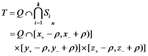 (4)
(4)
where x+ = max(x1, . . . , xm) , x_ = min(x1, . . . , xm)
y+ = max(y1, . . . , ym) , y_ = min(y1, . . . , ym)
z+ = max(z1, . . . , zm) , z_ = min(z1, . . . , zm)
From the Equation (4), we can deduce the position range through simple calculation in case of the k readers’ cell coordinates are known. With the appropriate parameters setting, the positioning precision can be high enough as we wanted.
3. Error Estimations and Comparison with Other Algorithms
3.1. Error Estimations in Positioning
Because the scope of communication has been simplified, the positioning error is inevitable, and this greatly influences the computing result. In order to simplify the calculation, we discuss this in 2 dimensional spaces.
Assume that a certain tag can be detected by two readers at the same time (see Figure 5). Defining the equations of G1and G2 as G1:x2+y2=32. G2 :(x-3)2+y2=32.
Obviously, the tag must be in the intersection Ω of G1 and G2
And
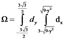 (5)
(5)
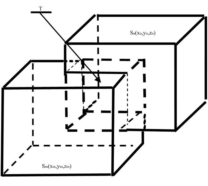
Figure 4. The intersection of two readers’ communication region (The cube T with dashed lines).
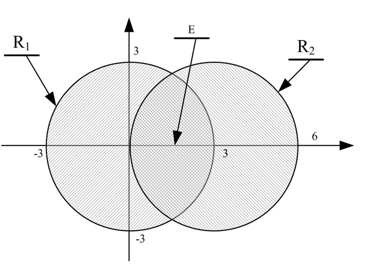
Figure 5. The real intersection of two readers’ communication region.
According to the simplified method, tag must be located in the intersection of E. The error event M can be described as the point whose position is in Ω (but not in E). The error possibility is p (M).
 (6)
(6)
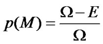 (7)
(7)
According to above equation, we can obtain the value of p (M) is about 17.3 percent, that is to say, when the two readers’ position are like Figure 6, only after excluding such errors can the algorithm work exactly.
In general, the estimated error is related to the positions of readers. For the same readers, if their positions are different, such error is different accordingly. If one tag can be detected by m readers, the calculation of estimated error is much more complicated than two readers, but we are sure that the error is a function of the positions m readers .We give the error definition as:
Definition 1: e(pr1,pr2,...,prm), where pri denotes the position of reader ri. e(pr1,pr2,...,prm) is
3.2. Comparison with Other Algorithms
We choose 3D RFID Positioning Algorithm [9], which is representative for 3d positioning, to be compared with 3D-PMWSN. The 3D RFID Positioning Algorithm is based on the location fingerprinting method. This method was first implemented in the RADAR system which is an RF-based indoor tracking system developed by Microsoft Research.
This positioning method achieves the best positioning results by two stages: the off-line training phase (off-line phase) and the on-line position determination phase (on-line phase). In the off-line phase, the received signal strength (RSS) from all the detectable transmitters and other relevant information including the physical coordinates

Figure 6. The simplified intersection of two readers’ communication region.
of the receiver, which are measured by other methods, such as using total stations or tapes, in the local coordinates, are collected at predefined reference points and stored in a database. The set of the database is called fingerprint. During the on-line phase the mobile user samples the RSS patterns and searches for similar patterns in the off-line database so as to find its most possible position.
Let’s compare the two positioning algorithms from four evaluation indicators.
1) Storage cost: As the nodes are relatively simple in Ad Hoc networks, any algorithm should be storage saved. Because there must be an off-line database, it is hard to setup such a database in the nodes of distributed system. But it is different for 3D-PMWSN; there is no off-line database, so the storage is saved.
2) Calculation complexity: for 3D-PMWSN, we can see from Equation (4) that the calculation in positioning is very simple. As to 3D RFID Positioning Algorithm, for the main calculations come from the search of off-line database, so the calculation is relatively simple. But this is based on the expensive cost of storage requirement, which is unsuitable for distributed Ad Hoc Networks.
3) Positioning accuracy: As to 3D-PMWSN, the positioning precision can be set according to the size of positioned object, which means the cell could be big or small. Nevertheless, the positioning resolution rate could not be changed for 3D RFID Positioning Algorithm because it is positioned by RSS.
4) Stability of the algorithm: In practice, the signal strength of RF transceiver is variable, which is to say the signal strength changes with the power supplied. For 3D-PMWSN, only using two states—tag detected or not, the influence of signal strength is little. The algorithm can work as long as a tag is captured by readers. But it is different for 3D RFID Positioning Algorithm. Because the positioning is mainly depended on signal strength, the signal attenuation, which may greatly increase the amount data of off-line database, may have great influences for positioning precision.
From above discussion, we can conclude that the 3D-PMWSN is better than 3D RFID Positioning Algorithm in positioning; especially for distributed Ad Hoc systems (see Table 1).
4. Simulation and Analysis
In order to evaluate the locating precision and rate of convergence, we do this simulation. Assume the number of readers is k, let the initial value of k be 2, and each reader’s cell coordinate are given as below. The simulation process is as following step
Step 1: us Definition 1 and exclude the positions that could cause errors.
Step 2: by using Equation (3), we can easily know the intersection size by the number of cells contained in it.
Step 3: increase k by step length 1.
Step 4: repeating from Step 1 to get a new intersection number until to one we consider suitable, then stop the calculation.
We choose two kinds of solutions .The emulation results are as bellows
Solution 1
Let s=10000, n=5000, r=100, using Equation (1), we can obtain ρ=28.
Let the reader’s number k be 10 and each cell’s coordinate is as follows:
R1(1305,1505,1805), R2(1310,1510,1810)
R3(1315,1515,1815), R4(1320,1520,1820)
R5(1325,1525,1825), R6(1330,1530,1830)
R7(1335,1535,1835), R8(1340,1540,1840),
R9(1345,1525,1825), R10(1350,1530,1830)
Firstly, we calculate the intersection of R1 and R2, and the result is about 68 thousand cells. Then, increase the reader number step by step. For R1, R2 and R3, the result is 47 thousand cells. When k increases to 9, the result is about 200 cells, which is very small compared with that k is 2.In practice, how many readers be chose is mainly based on the size of located object and cells in G. Accordingly we can choose appropriate parameters to get the result we need (see Table 2).
Solution 2
Let s=10000, n=2000, r=100.Then, we can deduce ρ= 12. Apart from the difference of cell numbers in G, other parameters are same as those in solution 1; the result is in Table 3. We can see that when k increases to 5, T has decreased to 27 cells.
For solution 1, we can conclude from Table 2 that the result T decreases as k increases, which means that the locating precision increases as k increase. Scattering 9 readers in G can get the precision degree to 100 grids.
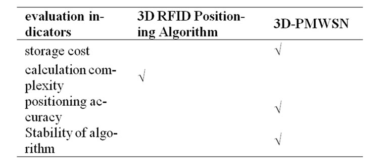
Table 1. The comparison of 3D RFID positioning algorithm and 3D-PMWSN (√-denotes the better one of evaluation indicators between two algorithms).
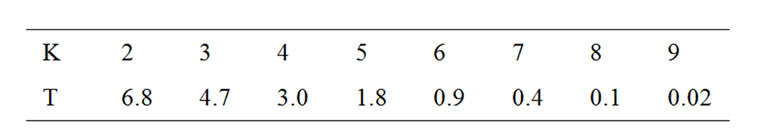
Table 2. The simulation result of solution 1 (the unit of T is 10 thousand cells).

Table 3. The simulation result of solution 2 (the unit of T is 10 thousand cells).
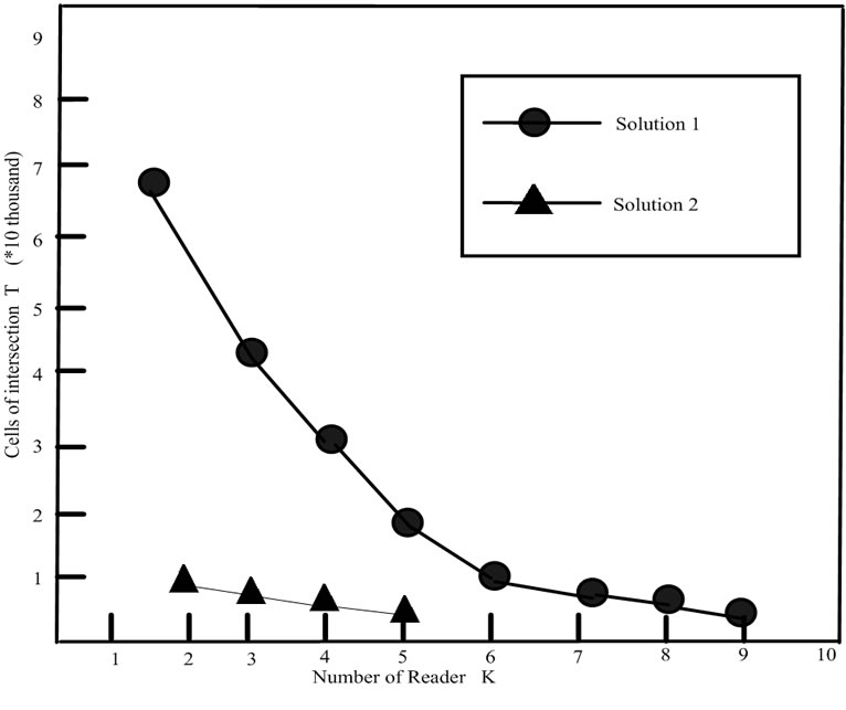
Obviously, the reader number does not need too much. So long as the positions are scattered suitably, the needed locating precision can be obtained. The algorithm is workable (see Figure 7).
For solution 2, the positioning speed is fast than solution 1, using only 5 readers .The reason is that the size of cell in solution 2 is bigger than that of in solution 1.It is to say that the positioning speed becomes faster in case of the resolution rate decreases. The positioning speed is faster by the cost of decreasing the resolution rate. In practice, a balance should be kept between these two facts.
5. Conclusion and Future Work
We gave a space cell concept in this paper and proposed a 3D-PMAHN model in Ad Hoc networks. An object’s position in 3 dimensional spaces can be computed by the given positioning algorithm. We also give the error estimation of the model. The simulation result shows that the 3D-PMAHN is simple and energy saving. Such characters meet the special requirements in Ad Hoc networks.
6. References
[1] F. B. Wang, L. Shi, and F. Y. Ren, “Self-localization systems and algorithms for ad hoc networks,” Journal of Software [J], Vol. 16, No. 5, pp. 857–866, 2005.
[2] X. Wei, J. W. Wan, and K. Huangfu, “New technique in single observer passive tracing based on particle filter,” Journal on Communications [J], Vol. 26, No. 12, pp. 81– 85, 2005.
[3] C. G. Tan and W. Y. Luo, “A survey of cooperation of nodes in mobile ad hoc networks,” Computer Science [J], Vol. 34, No. 4, pp. 23–27, 2007.
[4] S. N. Simic and S. Sastry, “Distributed localization in wireless ad hoc networks,” Technical Report UCB/ERL M02/26, Department of Electrical Engineering and Computer Sciences, University of California, Berkeley, CA, January 2002.
[5] J. Song, “Tracking the location of materials on construction projects [pHD],” The University of Texas at Austin, 2005.
[6] W. Ni and Z. X. Wang, “An adaptive multi-user location and tracking algorithm for indoor wireless network,” Journal on Communications [J], Vol. 26, No. 1, pp. 66– 73, 2005.
[7] L. W. Zhang and Z. H. Tan, “New TDOA algorithm based on Taylor series expansion in cellular networks,” Journal of Communications [J], Vol. 28, No. 6, pp. 7–11, 2007.
[8] L. W. Zhang and Z. H. Tan, “New 5TDOA algorithm based on Taylor series expansion in cellular networks,” Journal on Communications [J], Vol. 28, No. 6, pp. 8–12, 2007.
[9] K. F. Zhang, “Lecture notes in geoinformation and cartography,” pp. 374–38, 2007.