iBusiness
Vol.2 No.2(2010), Article ID:1959,5 pages DOI:10.4236/ib.2010.22021
Analysis and Evaluation for Core Competence of Insurance Company Based on SEM
![]()
1Department of Mathematics, Wuhan University of Technology, Wuhan, China; 2Department of Accounting, Chongqing Technology and Business University, Chongqing, China.
Email: tonghengqing@126.com, yeyang19851016@163.com
Received March 28th, 2010; revised April 27th, 2010; accepted May 21st, 2010.
Keywords: Core Competence, Insurance, SEM, Algorithm
ABSTRACT
Evaluation the core competence reasonably plays an important role in the insurance company, it is related to whether the insurance can maintain a stable long-term competitive advantage or not, and whether obtain a stable long-term excess profits or not. In this paper, we select 6 first-degree indexes (including the core competence) and 28 second-degree indexes to evaluate the core competence of insurance company by Structural Equation Model (SEM), and analysis the relationships among the first-degree indexes. Besides, we use a new algorithm proposed by us to improve the calculation of SEM.
1. Introduction
The essential of competition among enterprises is scramble for the required resources of their survival and development of enterprises, the competitiveness of enterprises is the ability of enterprises to compete for resources [1]. Traditional competitive theory still can not make a satisfactory answer of the long-term ups and downs of Enterprise. However, the theory of the core competitiveness study the ability of optimal allocation of resources of enterprises from the short-term extends to long-term. And point out that in order to make sure the survival and development of corporate sustainability, we must have more ability of optimal allocation of resources. In other words, companies must have strong core competitiveness.
The core competence was first proposed by C. K. Prahalad and Gary Hamel [2]. This theory is a kind of business strategy concept and paradigm which has great vitality; it opened the real password of the modern business success in a sense. Enhance the core competitiveness have great strategic significance for the development of the insurance business. Insurance companies operate with the characteristics of debt, once the insurance companies have poor core competitiveness, poor operating performance and unable to bear the compensation or payments, they will harm the vital interests of the insured, and even affect the stability of the whole society. So it is very significant to study the core competence of insurance company.
The core competence of insurance company is different from the general company. Professor J. P. Jan believes that the following 3 reasons account for this phenomenon. First, the insurance company cannot establishment the core competence rely on market segmentation or monopoly. Second, insurance products cannot apply for a patent. Third, regulatory authorities require the insurance company provide the transparent and open information of the insurance products for financial supervision [3]. Based on this features, many scholars establish the model to evaluate the core competence of insurance company. Such as DEA data envelopment analysis model, BSC (Balanced Score Card model) [4] and so on. Among the most important and most widely recognized model is FCEM (Fuzzy Comprehensive Evaluation Model) [5]. However, all of the above models are very subjective in a sense. In this paper, we introduce a model in which the coefficients and weights are calculated by samples, so it is more objective and convincing, and could offer more deep analysis for the index systems.
2. SEM for the Core Competence of Insurance Company
SEM is a rapid-developing embranchment of Application Statistics, which has a wide application in the area of Psychology, Economics and Sociology [6,7], especially in Customer Satisfaction Index (CSI) [8] model which is required by a series of ISO9000 criterions. This model not only studies the interior relationship among various factors, but also the relative and causal relations among latent variables. As we know, we cannot observe the value of the core competence directly. So it is a latent variable, and we can use the SEM to research.
Different companies have different competitive advantages; it may be different with the company’s industrial environment and strength. For example, Intel’s core competence is the chip manufacturing technology; CocaCola Company’s core competence is a trademark and formula, while Galanz’s core competence is the largescale and low-cost production capacity. The difference of the external environment and internal resources among the different industry is very large, so the constituent elements and cultivation methods of the core competence would be different with each other. Therefore, with the basic principles of selected index [9], we consider the specificity of the insurance enterprise; identified 5 firstdegree indexes which have relate to the enterprise’s core competence, all of them are latent variables. In order to study the core competence, we have to seek the observed variables for each latent variable. The variables are listed in Table 1 as follows:
There exists 13 relationships among the 6 structural variables (latent variables), which are expressed in Figure 1 (The relationships among variables are , expressed with dashed arrowheads; the relationships among independent variables are
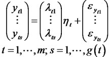
 , expressed with realline arrowheads). The structural relationship among the latent variables (structural model) can be put as follows:
As shown in the Figure 1, we can see the path relationships or causalities among these variables. Next we can express these causalities among the structural variables as equations as below:
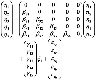 (1)
(1)
In general, suppose that  are
are ![]() dependent variables, arranging them as a vector
dependent variables, arranging them as a vector  by column as (1), that is
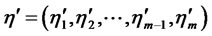 , we called it as endogenous latent variables; and
  are
are  independent variables, arranging them as a vector
  by column also,
 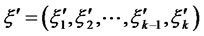 , we call it as exogenous latent variables. Then m × m square matrix
  is the coefficient matrix of
 , and m × k matrix
 ![]() is the coefficient matrix of
is the coefficient matrix of , let
, let  is the residual vector, then Equation (1) may be extended as:
 (2)
(2)
where  and
and .
.
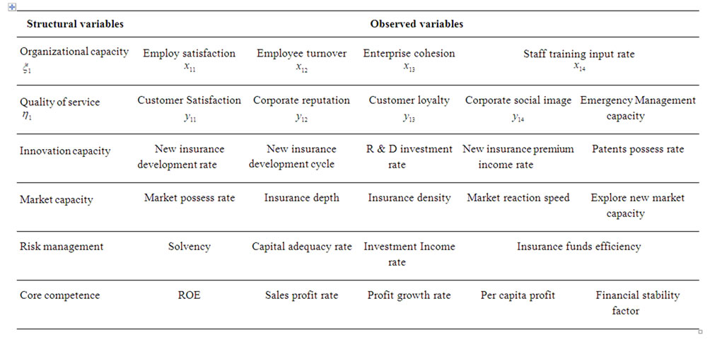
Table 1. Index of variables
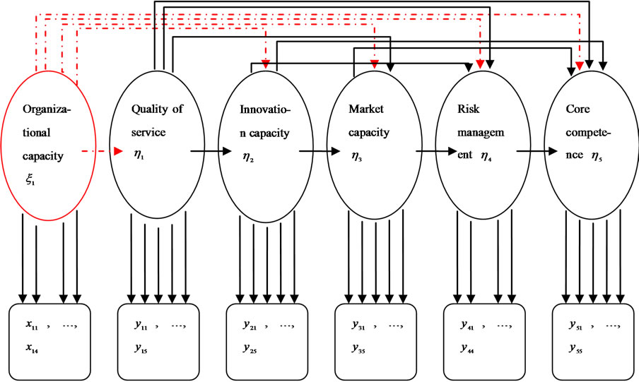
Figure 1. Path relationships among variables
There are always two systems of equations in a SEM. One is a structure system of equations among structural variables, and the other one is a measurement system of equations between structural variables and observed variables. From the above narrative, we can know the Equation (2) is the structure system of equations. And the structural variables are always implicit and cannot be observed directly. So there must have many observed variables to reflect the structural variables. And the relationships between the latent variables and the observed variables are the other equations of SEM, which are measurement system equations.
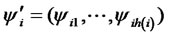
From the above, we know there are  exogenous latent variables and
 ![]() endogenous latent variables. Generally the observed variables corresponding to
endogenous latent variables. Generally the observed variables corresponding to  are denoted as
 ,
, ;
; , here
  is the number of observed variables corresponding to
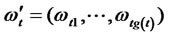
 . Similarly, the observed variables corresponding to
  are denoted as
 ,
,  ,
,  , here
  is the number of observed variables corresponding to
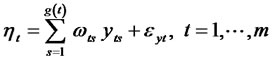
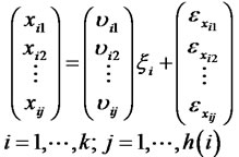
 . Then the observation equations in the Figure 1 can be expressed as the relationship from the observation variables to the structural variables:
 (3)
(3)
 (4)
(4)
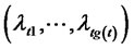
Where ,
,  are the summarizing coefficients, and
 ![]() with subscripts are random error items. Let
with subscripts are random error items. Let 
 ,
,  ,
,  ,
, . Then combining the Equations (2), (3) and (4) as:
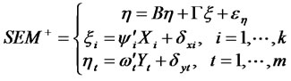 (5)
(5)
here  is the structural equations model with positive observation.
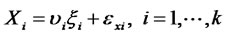
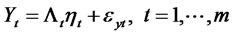
On the other hand, the measurement equations can be also expressed as follows:
 (6)
(6)
 (7)
(7)
here,  and
and  are the loading coefficients, and
 ![]() with subscripts are random error items yet.
with subscripts are random error items yet.
Let 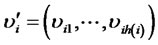 and the same time let
 . Then (5) and (6) can be expressed as:
 (8)
(8)
 (9)
(9)
Combine the Equations (2), (8) and (9), then we can get:
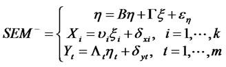 (10)
(10)
here  the structural equations model with converse observation.
3. Modular Constraint Least Squares Solution (MCLS)
We can skillfully use the least squares method in regression between each structural variable and its corresponding observation variables, and obtain the least squares solution of structural variable by the modular constraint of structure vector if we analyzing the observation equations of SEM carefully [10,11]. The algorithm for MCLS can be expressed as follows:
Algorithm 1. The MCLS of structural vector in .
.
Step 1 In , suppose
  all are unit vectors, we can calculate the least square estimates of the coefficients between each structural variable and its corresponding observation variables:
 (11)
(11)
where
 (12)
(12)
Similarly we have
 (13)
(13)
where
 (14)
(14)
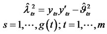
Step 2 In , calculate the least square estimates of structural variables by using of
 :
:
 (15)
(15)
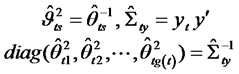
Step 3 In , make use of
  obtained in Step 2 to calculate the estimates of regression coefficients
  according to common linear regression method.
Step 4 In , make use of
  obtained in Step 2 to calculate the estimates of coefficient matrix
 .
.
Notice that (2) is a common linear regression equations, we can use the two-stage least squares method to calculate it.
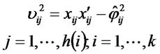
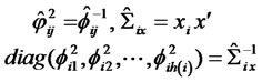
4. Definite Linear Algorithm with Prescription Constraint
According to the above algorithm, we can get the modular constraint least squares solution based on the constraints of the unit structural vector. But the solutions are not unique, and irrelevant to the modular length of the latent variables. As we know, it is not reasonable to stipulate that modular length of each structural variable is 1. If each modular length of the structural variable is not equal in possibly existing optimal solution set, then MCLS is not good.
An exploring way to improve the algorithm is to find a more reasonable constraint to replace modular constraint. After getting MCLS, we can change the modular length of structural variable in measurement system of equations to make the path coefficient between each structural variable and its corresponding observation variables satisfying prescription condition. That is:
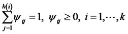 (16)
(16)
 (17)
(17)
Next, we compute the prescription condition from two cases.
If the corresponding path coefficients of MCLS are all non-negative at the beginning, we just need to divide a constant at the two sides of the Equation (3) and (4). This constant should be the sum of corresponding path coefficients in MCLS.
If the corresponding path coefficients of MCLS have negative at the beginning, we can not completely use the method of prescription regression [12]. However, we can change prescription condition and let ,
,  , here
  but not
 , and
, and  may be decided by user according to the actual problem. That is:
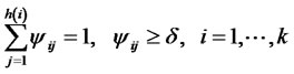 (18)
(18)
 (19)
(19)
If some initial regression coefficients are less than![]() , they are all changed as
, they are all changed as![]() , and the corresponding independent variables multiplied by coefficient
, and the corresponding independent variables multiplied by coefficient ![]() should be removed to the left of the equation in regression process.
should be removed to the left of the equation in regression process.
Under on these conditions we can continue to improve the algorithm of MCLS.
Algorithm 2. Improvement on Step 3 of the Algorithm 1 Step 3* After getting the estimated values as  of the structural variables
  in Step 2 of Algorithm 1, we calculate the summarizing coefficients
  by prescription regression, and next calculate the estimated values of
  again.
Step 3*.1 Define  in Step 2, and calculate
  in
in  by common regression.
Step 3*.2 For any , if
, if  (
( ) and
) and  for all
 . Then the both sides of Equation (3) are divided by
 . In the same way, the both sides of Equation (4) are divided by
  on the conditions.
After checking all , go to Step 4 in Algorithm 1.
Step 3*.3 For any , if there is
  or
or ![]() to make
to make  or
or  (
( ), then let corresponding item be fixed, that is
  or
or . The corresponding observation variables
  or
or  with its coefficient
 ![]() should be removed to the left of the equation, and combined with the latent variable
should be removed to the left of the equation, and combined with the latent variable  or
or  to regress, that is go to Step 3*.1 and Step 3*.2. After regression, the corresponding observation variable
  or
or  with its coefficient
 ![]() should be removed to the right of the equation.
should be removed to the right of the equation.
5. Final Remarks
In this paper, we propose SEM to analysis and evaluate the core competence of insurance company, and improve the algorithm of the SEM. It is more objective and scientific to use SEM in the evaluation of the core competence of insurance company compared with traditional methods, such as AHP, FCEM and so on, because the coefficients of this evaluation system are calculated by samples rather than designed arbitrarily. Therefore, we can have a better understanding the relationships among the indexes, which will do a great favor to decision-making analysis and evaluate for the core competence of insurance company.
REFERENCES
- Z. Q. Wang, “Study on Insurance Company Core Competence,” Southwestern University of Finance and Economics, Chengdu, 2007.
- C. K. Prahalad and H. Gary, “The Core Competence of the Corporation,” Harvard Business Review, Vol. 68, No. 3, 1990, pp. 79-91.
- J. P. Jan, “The Model Analysis of the Core Competence of Insurance Company,” Zhejiang Statistical, Vol. 2, 2004, pp. 20-22.
- J. Sun, “Study the Evaluation System of the Core Competence of Property Insurance Company,” Journal of insurance professional college, Vol. 23, No.1, 2009, pp. 37-42.
- M. J. Yu, “Evaluation Index System of the Core Competence of Insurance Company,” Tongling College Journal, Vol. 3, 2004, pp. 14-16.
- S. Y. Lee and X. Y. Song, “Model Comparison of Nonlinear Structural Equation Models with Fixed Covariates,” Psychometrika, Vol. 68, No. 1, 2003, pp. 27-47.
- S. Y. Lee and N. S. Tang, “Bayesian Analysis of Structural Equation Models with Mixed Exponential Family and Ordered Categorical Data,” British Journal of Mathematical and Statistical Psychology, Vol. 59, 2006, pp. 151-172.
- C. Fornell, D. M. Johnson and W. E. Anderson, “The American Customer Satisfaction Index: Nature, Purpose, and Findings,” Journal of Marketing, Vol. 60, No. 4, 1996, pp. 7-18.
- A. R. Xu, “Establish Evaluation Index System of the Core Competence of Insurance Company,” Statistics and Decision, Vol. 2, 2004, pp.12-13.
- Z. Q. Yang, “The Applications of Generalized the Least Squares Model,” Chinese Science Bulletin, Vol. 7, 1982, pp. 389-392.
- H. Q. Tong, L. Xiong and H. Peng, “Self-Organized Path Constraint Neural Network Structure and Algorithm,” Neural Information Processing, Part I, 2006, pp. 457-466.
- K. T. Fang, D. Q. Wang and G. F. Wu, “A Class of Constraint Regression-Fill a Prescription Regression,” Mathematica Numerica Sinica, Vol. 4, No. 1, 1982, pp. 57-69.