Journal of Geographic Information System
Vol.5 No.1(2013), Article ID:27928,13 pages DOI:10.4236/jgis.2013.51010
A Geographical-Origin—Destination Model for Calculating the Cost of Multimodal Forest-Fuel Transportation
LUT Savo Sustainable Technologies, Lappeenranta University of Technology (LUT), Mikkeli, Finland
Email: *olli-jussi.korpinen@lut.fi
Received November 14, 2012; revised December 15, 2012; accepted January 18, 2013
Keywords: Transportation; Forest Fuels; Railway; Waterway; GIS
ABSTRACT
As a consequence of increasing demand for wood fuels, the management of forest-fuel production chains has become an important logistics issue in Finland and Sweden. Truck-based transportation has been the dominant method in fuel supply from the areas around power plants. However, increasing demand has led to enlargement of supply areas and greater variety in supply methods, including also railway and waterway transportation. This study presents a GIS-based calculation model suitable for cost calculations for power plants’ forest-fuel supply chains. The model has multimodal properties—i.e., it provides transfer of forest-fuel loads between transportation modes—and enables case-specific adjustment of transportation and material-handling cost parameters. The functionality of the model is examined with a case study focusing on a region of intense forest-fuel use. The results indicate that truck transportation is competitive with railway transportation also for long transport distances. However, increasing the proportion of multimodal transportation for other than economic reasons (e.g., for supply security) could be reasonable, since the impact on total supply costs is marginal. In addition to honing of the parameters related to biomass availability and transport costs, the model should be developed through inclusion of other means of transportation, such as roundwood carriers.
1. Introduction
The EU has set a target of increasing the share of renewable energy sources (RES) in final energy consumption to 20% by 2020 [1]. In the most heavily forested EU countries, Finland and Sweden, wood fuels have an important role in meeting of the national targets, which are 38% for Finland and 49% for Sweden. Since the byproducts of wood industries are already used mainly for energy production purposes, the greatest wood-energy potential is found in forest fuels [2,3]. The term “forest fuels” refers to all technically and economically exploitable parts of trees that are unsuitable for timber or pulp and paper production. In Nordic forestry, these are branches and treetops as logging residues, stumps from clear‑cuttings, and small-diameter wood from young and dense forest stands.
Forest fuels’ supply can be divided into three parts: 1) forest operations; 2) transport operations; 3) materialhandling operations. In the first, the energy wood is harvested and forwarded to roadside storage, principally with machines similar to those used in roundwood harvesting. Transport operations include all transportation taking place via the road network and optionally also by rail and waterway. Besides moving of biomass from one carrier to another, material-handling operations include comminution of biomass. In addition to costs from these operations, the stumpage price, costs of storing the fuel at the roadside or terminals (e.g., interest costs), and costs created by supply management are usually included in supply-cost figures.
From a geographical point of view, Finland and Sweden show similarities in their regional imbalances of forest-fuel supply and demand. While the heat and power plants in industrialized and densely populated areas represent the greatest demand, the most extensive forest reserves are found in rural areas. In these Nordic countries, this generally means that the balance of supply and demand is positive in the north and negative in the south. In comparison with, for example, fossil-fuel transportation, loads of wood chips tend to have low energy density, usually rendering their road transportation unprofitable over long distances. Compared with the main transportation method, by road on truck-trailers (Figure 1), the railway and waterway options are cost-efficient for tran-
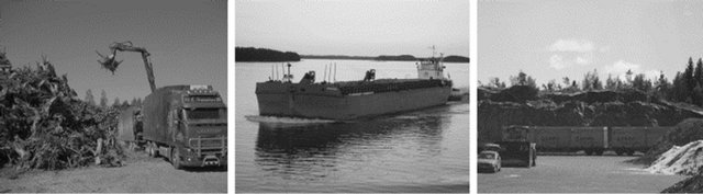
Figure 1. Example carrier types used in forest-fuel transportation. From left to right, a truck trailer loading stumpwood from roadside storage, a vessel unit of a barge and tugboat operating on an inland waterway, and chip-train wagons at a biofuel terminal.
sportation over longer distances, but, at the same time, they cause supplementary costs due to additional material-handling phases. According to findings of earlier studies on forest-fuel transportation (e.g., [4-6]), decisions on optimal forest-fuel logistics are always case-dependent, requiring geographical information about fuel availability, transportation networks, and prevailing or expected circumstances of other users’ demand. Because of the variety of supply methods and distinctive differences in the methods of roundwood supply, there have been requests for development of advanced calculation tools that are able to predict the economic outcomes of different supply cases.
This study presents a forest-fuel supply calculation model that has been designed for a GIS environment providing several options for selection of supply method, including all three transport networks: roads, railways, and waterways. With regard to multimodality and data of transport networks, this model resembles the linear optimization models that are used for developing roundwood supply [7,8], and today also forest-fuel supply [9,10] with a national scope in Finland and Sweden. In a departure from the nationwide perspective of previous models, this model is designed primarily for cases of single demand points as destinations, taking into more precise account the local properties of, for example, availability and competition related to the biomass to be transported. The model is divided into semi-automatic calculation steps. Automation saves time in repetitive calculation procedures and, consequentially, allows for sensitivity analyses of carrier selection, transport costs, selection of materialhandling machines, etc. In addition to the model’s structure, this paper presents a case study wherein the calculation model was used for analyzing the economic importance of railway transportation in an area of intense competition of forest fuels. The paper concludes with interpretation of the case study’s results and discusses the benefits and weaknesses of the model, as well as its applicability.
2. Material and Methods
2.1. Source Data and Geographical Extent
The source data consisted of municipal estimates of forest-fuel availability, several studies of transport and material-handling costs, and geographical datasets for transport networks and land-use data. Despite the model being applicable in theory also for other countries (e.g., Sweden) or even for transnational analyses, the geographical extent was confined to continental Finland, because of the limited availability of source data. The datasets were imported to a GIS environment, which was handled by ArcGIS® software.
2.2. The Geographical Grid and Origin Points
The origin points of forest-fuel supply were generated through a 2 × 2 km grid. The midpoints in the grid were extracted for further use in transportation analysis. This raster-to-vector conversion was required for connecting the estimates of availability of biomass to the transport network in vector form. The origin points represented roadside storage locations as places where forest operations end and the transport and material‑handling operations begin. In practice, there may be several roadside locations in a 4 km² area. From year to year, exact storage locations change as new cuttings appear. It was assumed that a precise geographical location is not necessary when the distance between an actual roadside location and the closest origin point in the model would be 0.0 - 1.4 km. Instead, describing the information on several roadside storage areas as attributes of one origin point reduces the load on route calculation processes. Another advantage of a network of fixed points is that it accepts source data in different formats. For example, the availability of small‑sized energy-wood potential is typically assessed from growing stock, and geographical information is given as polygon features with harvestable volume and area as attribute values. Hence, the values of the polygon features whose center points are in the same grid cell are summed for the corresponding origin point. On the other hand, logging residues and stumps are usually estimated from logging data via biomass conversion functions and selection criteria for forest stands suitable for energy-wood harvesting. Instead of polygons, the locations of logging data are usually roadside storage points whose values can be summed for the grid points as well.
2.3. Biomass Availability Analysis
2.3.1. Biomass from Regeneration Fellings
In Finnish forestry, logs are harvested from regeneration fellings and also, to a lesser extent, from thinnings [11], while the feasible logging residue and stump extraction is related only to regeneration fellings [12,13]. On the other hand, regeneration fellings produce some pulpwood too. In terms of harvest volumes on a local scale, correlation can be found between the volumes of harvested logs from all kind of stands and the volumes of all roundwood harvested from regeneration fellings [11,14], With this background, the biomass data were obtained from roundwood logging statistics reported by the Finnish Forest Research Institute [15]. Average roundwood cuttings from 2004 to 2008 were linked to municipal borders from 2008. There were 399 municipalities in continental Finland in 2008, with land area ranging from 6 km2 to 17,333 km2. One value for each tree species—i.e., the annual volume of logs harvested—represented each municipality. In practice, Finnish forests are dominated by three tree species: Scots pine (Pinus sylvestris), Norway spruce (Picea abies), and birch (Betula pendula or Betula pubescens). Of these species, the least dominant, birch, was removed from this part of the analysis, because logging residues and stumps are obtained mostly from coniferous forests. The roundwood volumes of pine and spruce were converted to logging residue and stump volumes by means of biomass conversion factors based on earlier assessments [12,16-18] (Table 1). The volumes were then cropped by a 70% recovery rate given in guidelines for sustainable energy-wood harvests for regeneration fellings [19].
The analysis produced two theoretical estimate values for each municipality: 1) harvest potential of logging residues; 2) harvest potential of stumps. Since the technically and economically viable harvest potential is less than the theoretical potential, a conversion factor of 0.40 for logging residues and 0.37 for stumps was used for gauging techno-economic potential [20]. The factors were principally based on the experience that some remote stands do not interest harvest operators, mainly because of high costs of harvesting or forwarding (i.e., off-road transport to roadside storage).
2.3.2. Biomass from Young Forest Stands
The availability analysis for harvestable biomass from young stands was based on the National Forest Inventory data collected by the Finnish Forest Research Institute. The availability analysis has been reported upon in terms of techno-economic harvest potential by municipality in 2008 [22,23].
2.4. Land-Use Data
Municipality-level estimates of biomass availability were assigned to origin points via a method utilizing land-use data in raster format [24]. First, the value for a municipality was divided evenly over the origin points such that the sum of the values equaled the municipal estimate. Then, proportional values for forest area in grid cells were calculated by means of raster analysis. GRASS GIS software was used in the raster analysis. The analysis exported a proportional value that was used for distribution of the values within the municipality. The average
Table 1. Biomass conversion factors for energy-wood harvests from regeneration fellings [12,16-18]—Northern Finland consists of the three northernmost provinces [21].
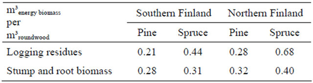
proportion of forest area in the municipality was used as the reference value. As a result of this method, the origin points in the most heavily forested areas of the municipality got higher estimates than those with less forest land. In the land-use data, the forest area stated represents all forest areas where the average annual capability of producing solid‑stem volume increment was more than 1 m3·ha−1 [21]. In addition to all urban and agricultural areas, stunted peatlands were counted as areas with no potential for harvests.
2.5. Transport-Network Analysis
2.5.1. The Multimodal Transport Network
The purpose of the transport-network analysis was to: 1) create a geographical layer of demand points that consisted of existing and planned demand points in Finland with expected annual forest fuel use of at least 360 TJ·a−1; 2) build a transport network with connectivity to the demand points. A multimodal network dataset was built from three vector layers, representing road, railway, and waterway networks. The source for the road-network layer’s data was Digiroad, a national road and street database maintained and kept updated by the Finnish Transport Agency [25]. Railway and waterway networks were extracted from the Topographic Database of the National Land Survey of Finland. The railway network included as an attribute value the status of electrification. Roadnetwork data included, for example, speed limits and oneway traffic restrictions. Waterway data covered inland waterways with a draft of 4.2 m. The waterway data had no additional attribute values.
To enable multimodal functions of the network dataset, places for transfers from one network to another were defined. The forest-fuel demand points with rail or water connection were automatically transfer sites for unloading purposes. The selection of other transfer sites—i.e., loading points for trains and vessels—was based on recommendations as to the most suitable loading locations and terminals for railway transportation of roundwood [26] and a development study of navigation on inland water-ways [27].
2.5.2. Costs of Truck-Based Transport
The economy of transportation is a sum of route-lengthdependent and independent costs. Ranta and Rinne [5] reported that the cost of forest fuel’s truck transportation is EUR0.28 - 0.56 GJ−1 already at the beginning of each trip when forest fuels are transported on Finnish roads. For chip-truck transportation, the cost function was
 (1)
(1)
where Cct is the cost of chip-truck transportation in EUR GJ−1 and dr is the shortest driving distance by road in kilometers from the origin to the demand point.
A truck (of the type shown in Figure 1) designed for transporting uncomminuted forest fuels is called an energy wood truck. The cost function used for these trucks was
 (2)
(2)
where Cewt is the cost for energy-wood truck transportation in EUR GJ−1 and dr is the shortest driving distance by road in kilometers from origin to demand point.
The cost functions were calculated for truck-trailers with a total weight of 60 tons, which is the maximum weight allowance in Finnish and Swedish road traffic [28, 29]. It was assumed that, in transportation of forest chips, the average payload is 44  [30] and when one is transporting uncomminuted biomass, the average payload is 33
  [31]1. In both functions, returning of empty trucks was included in the costs.
The cost functions were added to the calculation model in two parts. In the first part, two attribute-value fields were created in the road-network database, and these new fields received their values from the shape length multiplied by the corresponding coefficient for truck type—i.e., 0.0075 or 0.0097. Accumulation of these shape values was a crucial part of the route calculation. The second part involved adding the constant cost value (0.37 or 0.54) to the accumulation. This was done through definition of an added-cost-point barrier [32] for the demand point. The barrier allowed traffic to the end point only by adding of the constant cost value to the route properties (Figure 2).
2.5.3. Material-Handling Costs
Chip-truck transportation is the usual method of forest fuels’ transportation in Finland [31,33]. In this method, biomass is chipped at the roadside. The method is viable for logging residues and small-diameter wood but not for stumps. For comminuting the thick rootstock, operations require heavy crushers, which usually are unable to work at the roadside. The cost of roadside chipping depends slightly on the type of fuel [34]. In this model, an average value of EUR0.83 GJ−1 [35] was used as a default. This cost parameter was included in the route calculation, but, instead of origin point (i.e., the roadside), the action was determined for the point barrier that was already set as
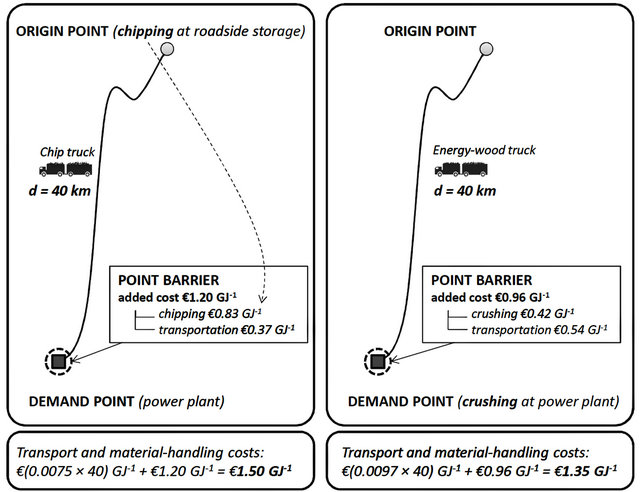
Figure 2. Example of unit costs’ calculation for two supply methods: roadside chipping (left) and crushing at the power plant (right). Costs that do not depend on the transport distance are added to the route at the point barrier at the demand point.
the constant in truck transportation costs.
Whenever crushing is used as the only option (for stumps) or the most convenient one (other forest fuels) for comminution, energy-wood trucks are needed for transportation. Crushing usually takes place at demand points, at least if they are equipped with stationary crushers. In other cases, a mobile crusher is used. This applies also for more complex systems wherein a terminal is used for storing, comminuting, and blending purposes. The unit costs of crushing depend greatly on the utilization rate [35]. Besides forest fuels, power plants commonly use other biomass to be crushed, such as waste wood, which keeps the crusher’s utilization rate high. In addition to annual operating time, mobile crushers’ operation costs depend on, for example, the distances between the terminals where they operate. According to Rinne et al. [35], EUR0.42 GJ−1 is the approximate crushing cost for a power plant with a stationary crusher when the annual crushing volume is 1.3 PJ. This was used as a default value for demand-point barriers whenever roadside chipping was not used. A mobile crushing cost of EUR0.92 GJ−1 was applied as the default for all supply methods involving terminal handling. This cost value represented a terminal where approx. 360 TJ of biomass is crushed annually [35]. For multimodal transport chains, further cost-point barriers were added for all possible loading points. The loading points featured a cost of EUR0.50 GJ−1, the difference between at-terminal costs and the crushing cost at the power plant.
It is worth mentioning that, unlike the cost values saved in the route layer, the model enables changes to the default values set for point barriers. This is advantageous for calculation tasks such as those for which case-specific, and more detailed, data are available rather than universal estimates. For example, if there is no rail connection at the power plant but a short transfer from the closest railway terminal to the power plant by truck, this transfer could be modeled by increasing the cost at the point barrier by the estimated further cost caused by truck transfer.
2.5.4. Waterway and Railway Transport Costs
Waterway and railway transport costs were added to the model similarly to the costs of road transportation. It was assumed that the transportation by water would be conducted by vessel units consisting of barges and tugboats. This was based on a study reporting the economy of this transport method [36]. The cost function was
 (3)
(3)
where Cww is the cost of waterway transportation in EUR GJ−1 and dww is the shortest waterway distance in kilometers from the loading point to the demand point. The expected carrying capacity of the vessel unit was 1500 , equating to 11.3 TJ2.
In Finland, availability of public reports about railway transportation costs is poor, and costs of railway transport services are difficult to predict. From a technical standpoint, transfers from diesel to electric power and vice versa are usual in Finland because the railway network is only partially electrified. A particularly large share of operation is that of yarding-in-transit, in which unit costs depend on the overall output of each rail yard. Furthermore, Finland’s rail freight traffic is open for competition, but the state-owned company, VR Transpoint, is still the only operator. The monopoly position means that, instead of distance, the pricing of freight services is based on competition with other modes of transportation, such as truck freight services [38]. The pricing is therefore very case-specific. The calculation model was unable to take into account complex price-fixing. A linear cost function was formed from sample data, which were collected from various transport cases. The cost function was
 (4)
(4)
where Crw is the cost for train transportation in EUR GJ−1 and drw is the shortest railway distance in kilometers from loading point to demand point. Accordingly, the train transportation costs given in this paper represent more the pricing itself than the operation costs for the service provider. It was assumed that the optimal train length would be 10 wagons, with each carrying three chip containers [39]. The total carrying capacity of a train was assumed to be 500 m³solid, which corresponds to 3.8 TJ.
2.6. Steps in the Calculation
2.6.1. Service-Area Queries
The first part of the calculation procedure was a service-area query for the selected demand point. Servicearea analysis is typically used for assessing the coverage areas of commercial services. In this case, the aim was to determine the size of the forest-fuel supply area for a given volume of forest-fuel demand.
This step included calculation of several service areas, starting with an area in which all parts of the network are within a 2 km driving distance. This was repeated with the range increased by 2 km until the maximum distance set3 was reached. Each service-area query took the sum of forest-fuel availability from the origin points that were no more than a kilometer from the roads shown in the road layer of the service area. Other points were rejected because of the assumption of poor economy of forest operations far from roads. The output was a table of service areas, with driving ranges and forest-fuel availability volumes as attributes. With this table, appropriate calculation distance for the next step in the calculations could be obtained.
2.6.2. Origin-Destination Route Matrix with Route Optimization
When the correct extent for the supply area was found, a route calculation was carried out by finding of the shortest routes from the origin points to the demand point. Because truck-transport costs were determined by route length (e.g., Figure 2), these routes were also the most profitable ones for supply methods based completely on direct transport by road to the power plant. In addition to the costs of these methods, the model calculated the costs of the most suitable multimodal transport options by adding up the costs of energy-wood-truck transportation to a loading point, costs defined for the point barrier at the loading point, costs derived from train or waterway transportation, and costs determined for the demand point. Examples of cost calculation for multimodal transport routes are presented in Figure 3.
The added-cost-point barriers were created for both loading and demand points, with the demand point displaying the same attributes as if the energy wood were transported directly to the plant. The loading points represented additional distance-independent4 costs of using train or waterway systems. By proceeding thus, the model was to select whether it was more economical to use a train or waterway option or transport the uncomminuted biomass directly to the plant. The output was a route matrix (Matrix B in Figure 4) that could include both direct and indirect routes for transportation of uncomminuted biomass. For the comparison with chip-truck transportation, a more complex method was needed, be-
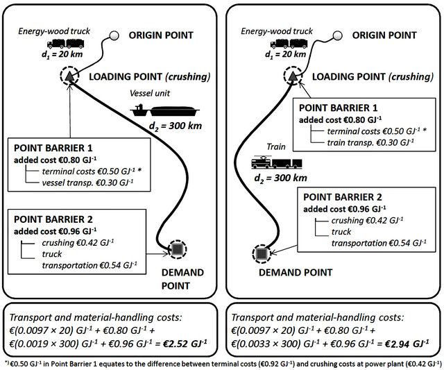
Figure 3. An example of unit cost calculation for multimodal supply methods: a method including waterway transportation (left) and a method including railway transportation (right). Costs that do not depend on the transport distance are added to the route at point barriers at loading and demand points.
cause of the differences in cost functions between truck types. This calculation step had two parts: The first part was calculation of the route matrix for energy-wood trucks, as explained above. In the second part, a route matrix allowing only chip-truck transport was calculated for the same area (Matrix A in Figure 4). These matrices were then compared record by record, and the best route for each fuel from each origin point was then saved to the final route matrix. For calculation of total transportation distances and costs, the distances for the individual routes were finally multiplied by the biomass volume available at the origin point and divided by the solid-content-carrying capacity of the respective carrier.
2.7. Case Study in the Selection of Alternative Transport Methods
2.7.1. The Case Study
The calculation model was used for choosing the optimal combination of supply methods for two CHP plants in Jyväskylä, Central Finland (62˚13'59''N, 25˚43'59''E). Total forest-fuel use at these facilities is 2.2 - 2.5 PJ·a−1 at present. The power plants’ energy production potential indicates that the demand for forest fuels could more than double from the current figures.
The main objectives in the case study were to: 1) determine the economic basis for railway transportation in an area of intense competition of forest fuels; 2) clarify the railway system’s influence on average supply costs in different demand conditions. Jyväskylä is an important logistics point on four railway lines, and the power plants in the study have a rail connection, in both cases about 5 km from the main railway station. The case study focused only on transportation and material handling between the origin and demand points, which means that, for example, shunting and unloading phases at the demand point were excluded.
The power plants were treated as a single demand point because they are near each other and owned by the same company. Based on the current and potential forest fuel use, three demand scenarios were used: 1) 2.5 PJ·a−1; 2) 4.3 PJ·a−1; 3) 5.4 PJ·a−1. To include train transportation as a supply option, we selected one loading location in the multimodal transport network for the case. The Haapajärvi rail yard (63˚45'00''N, 25˚19'59''E), 211 kilometers north of Jyväskylä by rail, was chosen because of the low local demand for forest biomass and spacious facilities for loading operations. Another advantage with this selection was that the railway route from Haapajärvi to Jyväskylä did not involve any additional yarding-intransit or locomotive exchange.
2.7.2. Biomass Availability for the Power Plant
The biomass availability analysis was carried out as described in Subsection 2.3 but with additional limitations to the estimated availability volumes. The first limitation was related to the availability of small-diameter wood. In addition to transport and material‑handling costs, supply costs include roadside price, which is composed of the given fuel’s stumpage price and costs of harvest operations5. The roadside prices of the three fuel types focused upon differ from each other, because of factors such as
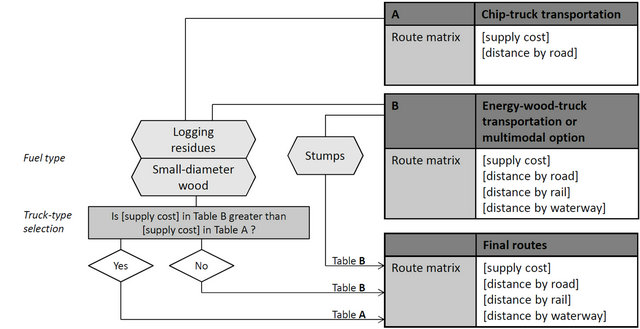
Figure 4. Intermediate route matrices for chip-truck transportation (A) and other transportation methods (B), and the conditions of selecting the most economical routes for the final route matrix. The variables required for calculation of total results for the analysis are presented in parentheses.
differences in harvest techniques and costs. On average, the roadside price is lowest for logging residues and at its highest for small-diameter wood. Production of fuel from small-diameter energy wood is partially supported by the government, with subsidies of EUR1.11 GJ−1 [10,18]. However, the national budget sets a ceiling for subsidy totals. Thus, subsidizing harvest for the full techno-economic potential would not be possible. Because of the restriction in the financial support from the government, a 50% limitation was set to the techno-economic availability of small‑diameter wood (see Section 2.3.2).
Secondly, it was assumed that the power plants in the case together have a roughly 25% market share in biomass trade in the region around Jyväskylä, while the existing local forest-fuel demand around Haapajärvi is mainly from small-scale use. The techno-economic availability at the origin points was reduced by 75%, with the exception of those points within a 60 km driving distance of Haapajärvi, where the limitation based on the market situation was defined as 25%.
Figures 5 and 6 present the availability of forest fuels in the areas under study as theoretical potentials and potentials after techno-economic and market-position-ba-sed reductions. The supply analysis in the case study was based on availability volumes presented as “potential after market-share cuttings”.
2.7.3. Supply Analysis
Of the three forest-fuel types, logging residues and smalldiameter wood were combined into one category for analysis because of the similarity in their various transport and material-handling methods. Stumps were treated as a
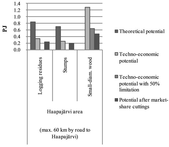
Figure 5. Forest-fuel availability in the Haapajärvi area in view of the limitations set in the analysis. The 50% limitation of techno-economic potential is based on expected insufficiency of national subsidies for small-diameter energy-wood production.
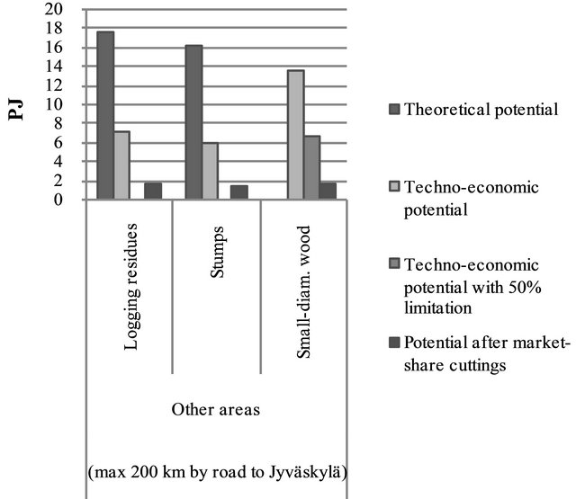
Figure 6. Forest-fuel availability in the study area outside the Haapajärvi area with the limitations used in the analysis. The 50% limitation for techno-economic potential is based on expected insufficiency of national subsidies for smalldiameter energy-wood production.
separate category, because roadside chipping was not an option for stumps; in other words, stumps were loaded on an energy-wood truck unchipped, whether the truck was heading to a train terminal or straight to the power plant. Logging residues and small-diameter wood were transported directly to power plants by chip truck, but, because a mobile crusher at the train terminal could be used also for logging residues and small-diameter wood, shortrange transport from roadside to terminal was determined to be best done by energy-wood trucks. According to the route optimization model, logging residues and smalldiameter wood could also be transported in unchipped form to a plant equipped with a stationary crusher. This option was, however, ignored, because a power plant’s crusher with an expected processing capacity of 1.3 PJ·a−1 might be overloaded if all forest fuels were crushed thus. Since waterway transportation was not an option in this case and logging residues and small-diameter wood were handled as a single category, three supply methods were included in the model: 1) roadside chipping and direct chip-truck transportation to power plants (hereafter referred to as the direct chip-truck method); 2) direct stump transportation and crushing at the power plants (direct energy-wood truck method); 3) energywood truck transportation to loading terminals combined with crushing at terminals and train transportation (train method).
The optimal supply method from each origin point was selected through comparison of the costs arising from material handling and transportation. While the train transport cost for a 216 km route was EUR1.00 GJ−1 and the difference between terminal and crushing costs at a power plant was EUR0.50 GJ−1, the train method was chosen for stump transportation if transport to loading terminals was at least EUR1.50 GJ−1 less costly than a direct truck route to the demand point. The selection procedure was not, however, applied for points over 200 km by road from Jyväskylä6. From the origin points ruled out by this definition, the points in the Haapajärvi supply area within a 60 km radius were still included in the study, with the train method as the only supply option.
3. Results
All transportation between the origin points and the demand point was done by trucks when the annual demand of the power plants was 2.5 PJ. The average transport distance was 91 km, corresponding to a transport cost of EUR1.05 GJ−1 for chips and EUR1.42 GJ−1 for stumps. Of the total fuel supply, 27% was stumps and 73% chips created from logging residues and small-diameter wood. Nevertheless, the energy-wood truck represented 30% of the distance driven. Because of the lower load density, it had to make more trips than a chip truck if it was to transport the same amount of biomass. The most remote origin point in the supply area was 138 km by road from Jyvä- skylä, with a supply cost of EUR2.24 GJ−1. In this scenario, train transportation was not a profitable option at all.
When the annual demand was increased to 4.3 PJ, the marginal transport cost, EUR2.56 G·J-1, became so high that the train method was the most economical supply method from some origin points near the Haapajärvi loading point. Annual supply through the terminal was 29 TJ, corresponding to eight train deliveries per year. The average distance in road transportation was 117 km and the maximum distance 182 km. Chip-truck deliveries’ share of the total supply volume increased from the aforementioned 73% to 75%, reflecting the more advantageous cost function for the roadside chipping method with longer transport distances.
In the scenario with the highest fuel demand, 5.4 PJ·a−1, 74% of the volume was transported by chip trucks. The lower number of chip-truck loads was principally a consequence of the increased volume transported by train. The train method represented a 151 TJ supply volume, even though this was much less than the mobile crusher’s potential capacity (360 TJ·a−1) at the loading terminal. Also contributing to chip transportation’s slightly lower share was that the limiting transport distance of 200 km with the direct chip-truck method was reached when the supply exceeded 5.3 PJ. Therefore, all deliveries whose total supply costs were more than the marginal cost of the direct chip-truck method at 200 km (i.e., EUR2.70 GJ−1) were transportation by either the direct energy-wood truck method or the train method. The most expensive deliveries resulted in a supply cost of EUR2.72 GJ−1, which equates to a 181 km driving distance in direct energywood truck transportation or a 26 km distance to the loading terminal.
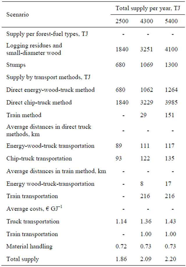
The main results of the case study are presented in Table 2. The average costs given for material handling include all costs of chipping, crushing, and terminal operations. Train transportation’s share of the total costs for a total supply of 4.3 PJ and 5.4 PJ was 0.3% and 1.3%, respectively.
Because only 151 TJ was allocated to train transportation, additional analysis was carried out in order to find the economic influence of increasing the biomass flow through the terminal to 360 TJ·a−1, which was the mobile crusher’s projected annual processing capacity. Therefore, the most expensive direct truck loads, corresponding to 209 TJ of energy in total, were either redirected to a loading terminal or replaced with the most profitable transport beyond the 26 km driving range from the terminal. As a result, the average supply cost for the whole
Table 2. Results in the case study.
supply scenario was increased by EUR2.70 TJ−1 (i.e., EUR0.0027 GJ−1). The enlargement of the supply area around Haapajärvi is shown in Figure 7, which also includes the geographical extent for the results presented in Table 2.
4. Discussion
4.1. The Case Study
The results of the case study indicate that railway transportation of forest fuels could be a viable alternative to direct truck-transport methods. Nonetheless, even in regions with intense competition of forest fuels, this conclusion holds only when very substantial amounts of forest fuels are to be transported. Direct chip-truck transportation is very competitive even with longer transport distances if the supply method is selected solely on the cost bases used in the study. In the additional scenario, 209 TJ of biomass was redirected from direct truck methods to the train method. Such redirection would be reasonable for, at least, the following reasons:
• The unit cost used for mobile crushing was initially intended for 360 TJ·a−1 productivity.
• Train transportation is probably unprofitable with low transport volumes, such as 151 TJ·a−1, unless concurrent use exists for the wagons utilized.
• It is sensible to use terminals for storing the biomass as a buffer against sudden disruptions in the supply system. The train method automatically includes terminal storage. The more biomass is stored at the terminal, the better the supply security is.
Usually, terminals are not accorded any concrete financial value for enhancing supply security. In the calculation model, this function should be compensated for by a negative cost attribute, but judging a suitable amount is difficult and case-specific. What is the likely-hood of a fuel shortage for a large-scale power plant using biofuels if there are no buffer terminals for backup, and how costly would it be to shut down the plant or use more expensive fuels, for example, in the middle of the
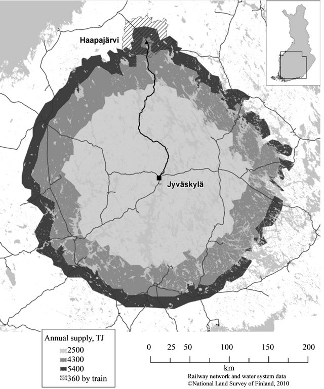
Figure 7. Forest-fuel supply areas in the scenarios used for annual demand.
heating season? In relation to the additional scenario of the share of the train method being increased to 360 TJ·a−1, the difference of EUR2.70 TJ−1 in average supply costs may be considered a low cost for increased supply security.
4.2. The Calculation Model
Despite the fact that waterway transportation was excluded, the case study showed that a geographical calculation model including multimodal properties is suitable for forest‑fuel transportation analyses insofar as transport alternatives are evaluated solely in economic terms. The cheapest means of transportation is found, and for most cases this is direct road transportation to the demand point. The case study also revealed that some distanceindependent costs in the model should not be considered to be completely fixed costs, because the utilization rates and the actual unit costs of crushers at terminals and power plants depend on the amounts of biomass that have been allocated to these points in the route calculation. The same applies to trains, whose cost functions should be unequal for different amounts of transported biomass, and even for different rail lines. Now, the basis for the train transportation cost function was a set of samples from other transportation cases, for which the annual number of train deliveries and transport volumes were unknown and the costs were more like supplier-set prices than dependent costs. In a comparable case study from Eastern Finland, Tahvanainen and Anttila [40] found that train transportation could be profitable even when the transport distance is 135 km or greater. That finding can be questioned because the costs used for chip trains were based on wagons used for roundwood transportation and the number of train-loading points was most likely exaggerated in view of the investment and maintenance costs of forest-fuel terminals [35].
In the biomass availability analysis, the method applied for weighting the municipality-level availability estimates with proportional forest-land area attributes was important because of the multimodal character of transport analysis. If truck transportation alone were employed for large-scale supply, the differences in forestfuel potential between individual origin points would probably even out in the final results. However, the supply areas around the loading points are so small that geographical differences within the municipalities matter. For example, if a train-loading point were surrounded by residential or agricultural land while the majority of the forests were further from the municipal center, which is usually the case, and if the origin points in the model had similar estimates of biomass availability, the calculation would result in excessively short average distances between the origin points and the loading point.
The source data for the availability analysis were based on roundwood logging statistics and results from forest inventory and were reprocessed such that the values for the origin points corresponded to the technoeconomic harvest potentials for each fuel. Techno-economic potentials should still be reduced in consideration of the competition of forest fuels. This was done in the case study via reduction of the potential with coefficients that were based on local knowledge of competition conditions. Adding an advanced calculation module to predict the conditions of competing demand points could probably give more reliability to the harvest potential figures. In Finland, studies of forest-fuel supply for multiple demand points (e.g., [10,41]) have generally used simple demarcation between power plants, but the supply areas of competing demand points actually overlap with each other in free competition. In case-specific supplyarea analysis, the competition should be modeled through definition of geographical rules that allow for overlap in the competition.
The analysis for multimodal transport networks focused on the supply methods most commonly used in Finland. Additional fleet alternatives for long-distance transportation were a bulk-load barge and a train carrying standard twenty-foot containers. Both of these methods necessitate the biomass being chipped before loading. However, since the energy use of small-diameter wood has recently increased [42], there would be a need also to include roundwood carriers in the model. In this study, all small-diameter trees were assumed to be harvested whole, which is the most profitable harvest method when chipping is done at the roadside [43]. This fuel source can also be harvested as delimbed stemwood, which results in higher harvest costs. On the other hand, delimbed wood can be transported from the roadside at a lower transportation cost via trucks and wagons as used in pulpwood transportation. Given the better cargo density and, especially, easier operations in trains’ loading and unloading, it can be assumed that transportation of delimbed small-diameter wood will increase as a consequence of the growth in forest-fuel demand nationwide and the increasing transport distances.
5. Conclusion
This paper presented a calculation model for selecting the most cost-efficient way of transporting forest fuels in different cases. The main focus of the paper was in presentation of the methodology, but a case study was also included to demonstrate how the model operates in GIS environment. Increasing demand for biofuels in the EU calls for more advanced planning and analyzing tools for logistics. This calculation model could be developed to include also other feedstocks, such as agro-biomass, and additional means of transportation. The model is also applicable for analysing supply-chain based emissions.
REFERENCES
- European Commission, “Directive 2009/28/EC of the European Parliament and of the Council of 23 April 2009 on the Promotion of the Use of Energy from Renewable Sources and Amending and Subsequently Repealing Directives 2001/77/EC and 2003/30/EC,” European Commission, Brussels, 2010.
- M. Pekkarinen, “Kohti vähäpäästöistä Suomea: Uusiutuvan Energian Velvoitepaketti,” Government’s Ministerial Working Group for Climate and Energy Policy, Helsinki, 2010.
- Å. Thorsén, R. Björheden and L. Eliasson, “Efficient Forest Fuel Supply Systems. Composite Report from a Four Year R&D Programme 2007-2010, Uppsala, 2011.
- H. Mahmudi and P. C. Flynn, “Rail vs Truck Transport of Biomass,” Applied Biochemistry and Biotechnology, Vol. 129, No. 1-3, 2006, pp. 88-103. doi:10.1385/ABAB:129:1:88
- T. Ranta and S. Rinne, “The Profitability of Transporting Uncomminuted Raw Materials in Finland,” Biomass and Bioenergy, Vol. 30, No. 3, 2006, pp. 231-237. doi:10.1016/j.biombioe.2005.11.012
- M. Gronalt and P. Rauch, “Designing a Regional Forest Fuel Supply Network,” Biomass and Bioenergy, Vol. 31, No. 6, 2007, pp. 393-402. doi:10.1016/j.biombioe.2007.01.007
- M. Forsberg, M. Frisk and M. Rönnqvist, “FlowOpt—A Decision Support Tool for Strategic and Tactical Transportation Planning in Forestry,” International Journal of Forest Engineering, Vol. 16, No. 2, 2005, pp. 101-114.
- P. Iikkanen, S. Keskinen, A. Korpilahti, T. Räsänen and A. Sirkiä, “Raakapuuvirtojen Valtakunnallinen Optimointimalli (a National Optimisation Model for Raw Wood Streams),” Research reports of the Finnish Transport Ageency, Helsinki, 2010.
- P. Flisberg, M. Frisk and M. Rönnqvist, “FuelOpt—A Decision Support System for Forest Fuel Logistics,” Proceedings of the 3rd International Conference on Information Systems, Logistics and Supply Chain, Creating Value through Green Supply Chains, Casablanca, 14-16 April 2010, p. 8.
- P. Iikkanen, S. Keskinen, A. Korpilahti, T. Räsänen and A. Sirkiä, “Energiapuuvirtojen Valtakunnallinen Optimointimalli (a National Optimisation Model for Energy Wood Streams),” Research reports of the Finnish Transport Agency, Helsinki, 2011.
- J. Hynynen, A. Ahtikoski, J. Siitonen, R. Sievänen and J. Liski, “Applying the MOTTI Simulator to Analyse the Effect of Alternative Management Schedules on Timber and Non-Timber Production,” Forest Ecology and Management, Vol. 207, No. 1-2, 2005, pp. 5-18. doi:10.1016/j.foreco.2004.10.015
- T. Ranta, “Logging Residues from Regenaration Fellings for Biofuel Production—A GIS-Based Availability and Supply Cost Analysis,” Ph.D. Thesis, Lappeenranta University of Technology, Lappeenranta, 2002.
- J. Laitila, T. Ranta and A. Asikainen, “Productivity of Stump Harvesting for Fuel,” International Journal of Forest Engineering, Vol. 19, No. 2, 2008, pp. 37-46.
- A. M. I. Kallio, P. Anttila, M. McCormick and A. Asikainen, “Are the Finnish Targets for the Energy Use of Forest Chips Realistic—Assessment with a Spatial Market Model,” Journal of Forest Economics, Vol. 17, No. 2, 2011, pp. 110-126. doi:10.1016/j.jfe.2011.02.005
- Finnish Forest Research Institute, “MetINFO. Forest-Related Information Services and Expert Systems,” Finnish Forest Research Institute, Helsinki, 2011.
- P. Hakkila, “Mechanized Harvesting of Stumps and Roots. A Sub-Project of the Joint Nordic Research Programme for the Utilization of Logging Residues,” Communicationes Instituti Forestalis Fenniae, Vol. 77, No. 1, 1972, P. 71.
- P. Hakkila, “Puuenergian Teknologiaohjelma 1999-2003, Loppuraportti,” Tekes, Helsinki, 2004.
- K. Kärhä, J. Elo, P. Lahtinen, T. Räsänen, S. Keskinen, P. Saijonmaa, H, Heiskanen, M. Strandström and H. Pajuoja, “Kiinteiden Puupolttoaineiden Saatavuus ja Käyttö Suomessa Vuonna 2020,” Publications of the Ministry of Employment and the Economy, Helsinki, 2010.
- O. Äijälä, M. Kuusinen and A. Koistinen, “Hyvän Metsänhoidon Suositukset Energiapuun Korjuuseen ja Kasvatukseen (Guidelines for Sustainable Production of Energy Wood),” Metsätalouden Kehittämiskeskus Tapio, Helsinki, 2010.
- M. Maidell, P. Pyykkönen and R. Toivonen, “Metsäenergiapotentiaalit Suomen Maakunnissa (Regional Potentials for Forest-Based Energy in Finland),” Pellervo Economic Research Institute, Working Papers, Helsinki, 2008.
- Finnish Forest Research Institute, “Finnish Statistical Yearbook of Forestry 2010,” Finnish Forest Research Instatute, Sastamala, 2010.
- P. Anttila, K. T. Korhonen and A. Asikainen, “Forest Energy Potential of Small Trees from Young Stands in Finland,” In: M. Savolainen, Ed., Bioenergy 2009—Sustainable Bioenergy Business. 4th International Bioenergy Conference from 31st of August to 4th of September 2009, FINBIO Publications, Helsinki, pp. 221-226.
- J. Hynynen, A. Asikainen and H. Ilvesniemi, “Bioenergiaa Metsästä—Metsiemme Bioenergiavarat ja Energiapuun Talteenoton Vaikutukset,” Energiapuussa Tulevaisuus Seminar, Evo, 2008.
- National Land Survey of Finland, “SLICES Database metadata,” 2006. http://www.maanmittauslaitos.fi/digituotteet/slices-maankaytto
- Finnish Transport Agency, “Digiroad,” 2010. http://www.digiroad.fi/dokumentit/en_GB/documents/
- P. Iikkanen and A. Sirkiä, “Rataverkon Raakapuun Terminaali-ja Kuormauspaikkaverkon kehittäminen: Kaikki Kuljetusmuodot Kattava Selvitys (Development of the Railway Raw Wood Terminal and Loading Point Network: Study Covering All Forms of Transport),” Research Reports of the Finnish Transport Agency, Helsinki, 2011.
- T. Sikiö and I. Salanne, “Saimaan Sisävesiliikenteen Kehittämisselvitys (Development Study of Inland Navigation on Lake Saimaa Area),” Publications of the Finnish Maritime Administration, Helsinki, 2008.
- Finland, “Decree on the Use of Vehicles on the Road,” The Finnish Law, Helsinki, 1992.
- European Commission, “Council Directive 96/53/EC of 25 July 1996 Laying Down for Certain Road Vehicles Circulating within the Community the Maximum Authorized Dimensions in National and International Traffic and the Maximum Authorized Weights in International Traffic,” European Commission, Brussels, 1996.
- J. Laitila, “Harvesting Technology and the Cost of Fuel Chips from Early Thinnings,” Silva Fennica, Vol. 42, No. 2, 2008, pp. 267-283.
- K. Kärhä, A. Mutikainen and A. Hautala, “Saalasti Murska 1224 HF Käyttöpaikkamurskauksessa (Saalasti Murska 1224 HF at Power Plant Crushing),” Metsäteho Tuloskalvosarja, Helsinki, 2011.
- Esri, “Desktop Help 10.0—Barriers,” 2012. http://help.arcgis.com/en/arcgisdesktop/10.0/help/index.html#//004700000056000000.htm
- K. Kärhä, “Metsähakkeen Tuotantoketjut Suomessa vuonna 2010 (Industrial Supply Chains of Forest Chip Production in Finland in 2010),” Metsäteho Tuloskalvosarja, Helsinki, 2011.
- T. Ihalainen and A. Niskanen, “Kustannustekijöiden Vaikutukset Bioenergian Tuotannon Arvoketjuissa,” Working Papers of the Finnish Forest Research Institute, Helsinki, 2010.
- S. Rinne, K. Karttunen, O.-J. Korpinen, T. Ranta and J. Handelberg, “Terminaali Liiketoimintana,” In: K. Karttunen, J. Föhr and T. Ranta, Eds., Energiapuuta Etelä-Savosta (Energywood from South-Savo), Lappeenranta University of Technology, Lappeenranta, 2010, pp. 125-145.
- K. Karttunen, E. Jäppinen, K. Väätäinen and T. Ranta, “Metsäpolttoaineiden Vesitiekuljetus Proomukalustolla (Inland Waterway Transport of Forest Fuels),” Research Report ENTE B-177, Lappeenranta University of Technology, Lappeenranta, 2008.
- E. Alakangas, “Suomessa Käytettyjen Polttoaineiden Ominaisuuksia (Properties of Fuels Used in Finland),” VTT Research Notes 2045, Technical Research Centre of Finland, Espoo, 2000.
- M. Mäkitalo, “Market Entry and the Change in Rail Transport Market when Domestic Freight Transport Opens to Competition in Finland,” Ph.D. Thesis, Tampere University of Technology, Tampere, 2007.
- O.-J. Korpinen, J. Saranen, E. Jäppinen and T. Ranta, “Evaluating the Suitability of Long-Distance Railway Transportation of Forest Fuels in Finnish Circumstances,” 18th European Biomass Conference and Exhibition, 3-7 May 2010, Lyon, pp.156-162.
- T. Tahvanainen and P. Anttila, “Supply Chain Cost Analysis of Long-Distance Transportation of Energy wood in Finland,” Biomass and Bioenergy, Vol. 35, No. 8, 2011, pp. 3360-3375. doi:10.1016/j.biombioe.2010.11.014
- T. Ranta and O.-J. Korpinen, “How to Analyse and Maximise the Forest Fuel Supply Availability to Power Plants in Eastern Finland,” Biomass and Bioenergy, Vol. 35, No. 5, 2011, pp. 1841-1850. doi:10.1016/j.biombioe.2011.01.029
- E. Ylitalo, “Puun Energiakäyttö 2010, Metsätilastotiedote 16,” 2011. http://www.metla.fi/metinfo/tilasto/julkaisut/mtt/2011/puupolttoaine2010.pdf
- J. Laitila, J. Heikkilä and P. Anttila, “Harvesting Alternatives, Accumulation and Procurement Cost of Small-Diameter Thinning Wood for Fuel in Central Finland,” Silva Fennica, Vol. 44, No. 3, 2010, pp. 465-480.
NOTES
*Corresponding author.
1By default, payloads for stump transportation as given by Kärhä et al. [31] were used as the reference for all fuel types.
2The ratio between the energy content and solid cubic volume is different for each fuel source, with the exact values depending on such factors as which wood density or moisture values are applied as defaults (e.g., [18,37]). In this study, it was assumed that the ratio is 7.56 GJ·m−3 for logging residues and small‑diameter trees and 10% higher (i.e., 8.32 GJ·m−3) for stumps. The carrying capacity is here converted to energy content with a 7.56 GJ·m−3 ratio.
3This was to be manually defined. The user of the calculation model was expected to have a sense of the geographical extent of large-scale supply of forest fuels.
4Distance-independent costs could be understood also as fixed costs and distance-dependent costs as variable costs. The terms “fixed costs” and “variable costs” also encompass business operations with no geographical sense, whereas the authors wanted to express the costs’ dependency on geographical properties explicitly.
5The spatial variation in roadside prices of all forest fuels is so great that the fuel types’ price ranges overlap each other [10]. Because of the uncertainty in the prediction of price differences between locations, roadside prices were excluded from the study. Given the study’s objectives and the finding that there were no great differences in small-diameter wood’s availability across the study area, ignoring the roadside price differences was not expected to have significant impact on the selection of supply method or on the sizes of supply areas in the case study.
6This demarcation was used because the cost functions chosen for truck transportation were assumed to be valid only for distances shorter than 200 km. There was uncertainty about how much a long transportation range affects such matters as scheduling of work shifts and the drivers’ compensation for overtime and, thus, the economy of transport opera- tors.