Journal of Geographic Information System
Vol. 4 No. 3 (2012) , Article ID: 19603 , 6 pages DOI:10.4236/jgis.2012.43033
Spatial Uncertainty Handling in Lake Extent Trend Analysis Using Remote Sensing and GIS Tools: The Case of Lake Naivasha
College of Engineering and Technology, University of Dar es Salaam, Dar es Salaam, Tanzania
Email: *julian@udsm.ac.tz
Received February 17, 2012; revised March 1, 2012; accepted March 11, 2012
Keywords: Image Objects; Spatial Uncertainty; Spatial Change Detection; Remote Sensing Time Series
ABSTRACT
This study presents an approach of handling spatial uncertainty of poorly defined objects when mapping, monitoring and trend analysis. The approach was tested using a series of Landsat ETM+ images of Lake Naivasha, Kenya, whose boundaries are fuzzy due to the presence of marshes and floating vegetation. In this approach image segments technically known as image objects were created and merged based on attributes such as segment size, location, Normalized Difference Vegetation Index (NDVI) and individual band contribution to the respective image segment. Then class labels were assigned to each image object rule-based fuzzy object image classification algorithm. Finally we calculated the spatial uncertainty in lake extent at a moment in time. Using the same parameters we classified a series of at irregular time interval images and performed time series analysis to identify trend in lake extent and explore the impact of uncertainty in lake extent definition. The analysis indicates that the lake extent is sensitive to threshold definition. At different thresholds, one is likely to interpret differently on the spatial increase or decrease. The varying size in lake extent at a moment in time is a result of temporal variations over water surface as a result of currents. This will always affect long term spatial change detection in spatial objects with fuzzy boundaries. We therefore conclude that this method provides a quick overview and highlights uncertainty related to image quality and time of observation. The next step will be to use multiple sensors representing the same object at irregular time interval as means of including redundant observations in long term analysis.
1. Introduction
Mapping the surface area of spatial objects on the surface of the Earth requires the handling of spatial uncertainty. This spatial uncertainty may originate from the definition of the spatial object within a class, the type of boundary (crisp or fuzzy), the accuracy with which it can be detected and the time and scale of observation. In studies of trends, such as change of size of glaciers as a result of climate change, or the shrinking of a lake due to increasing water extraction for irrigation, it is important to include the spatial distribution of uncertainty regarding the mapped feature for each date [1]. If both spatial and temporal uncertainties are known, a more reliable assessment of the trend can be made.
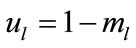
This paper presents an approach to include uncertainty of the mapped feature into multi-temporal analysis. The approach uses membership ml to the class “lake” as a measure of certainty for that class. The underlying assumption is that the combined uncertainty as a result of class definition, mixed pixels, gradual transitions, sensor characteristics and the classification is directly reflected in a decrease in membership for the class of interest. The uncertainty for lake, ul, is defined as in Equations (1) and (2) below
 (1)
(1)
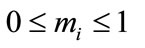
for all memberships mi for class i in a pixel and
 and
and 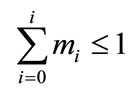 (2)
(2)
To demonstrate the approach, a series of Landsat 7 ETM+ images of Lake Naivasha, Kenya (Table 1) was used. Over the past decade, water levels and surface area of the lake have dropped, presumably because of larger water consumption by the people and agricultural activities along the shore as well as climatic changes [2]. The North-western part of the lake is surrounded by steep slopes, providing a relatively crisp boundary. In other areas the boundaries of the lake are gradual and include various types of marshes. Whether the marshes belong to the lake or the land is a matter of definition, as definitions depend on the type of vegetation and the length of time the marsh is actually flooded each year. Added vagueness comes from green algae and from free floating vegetation, which moves around the lake depending on the wind direction. The algae and floating vegetation increase the spectral confusion between the lake area and the surrounding vegetation classes [1].
2. Methods
2.1. Study Area Description
Lake Naivasha in Kenya has been used in this study (Figure 1). The lake is located at approximately 00˚45'00''S, 36˚21'00''E. It is situated in the West of Naivasha town in Kakuru District within Rift Valley Province. It is a shallow (mean depth of 6 m, endorheic, freshwater lake in warm and semiarid conditions in the eastern Rift Valley of Kenya, lying within an enclosed basin at an altitude of 1886 m above mean sea level with surface area fluctuating between 100 and 150 km2. It is world famous for its high biodiversity, especially for birds (more than 350 bird species) [3]. In the year 1995, Lake Naivasha was declared as Ramsar site (Wetland of International Importance) because of its diverse acquatic and terrestrial ecosystems.
The climate of this wetland area is hot and dry with a high potential evaporation exceeding the rainfall by around three times [4]. The area receives rainfall between April to June and October to December each year. The
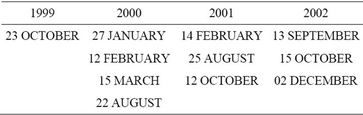
Table 1. Landsat ETM+ images of Lake Naivasha.
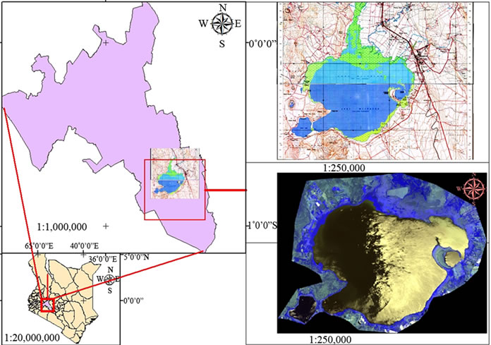
Figure 1. Location of study area and corresponding Landsat7 ETM+ image acquired on the 15 October 2002.
rest of the year is dry season.
The lake system has fringing swamps dominated by papyrus and submerged vegetation and an attendant riverine floodplain with a delta into the lake. These swamps vary in size especially during the rainy season resulting into uncertainty in lake/water boundary. In addition, there are acquatic plants (water hyacinth) that live and reproduce freely on the surface of fresh water or can be anchored in mud. There are also other submerged vegetation species. The presence of these types of vegetation makes the delineation of water/land boundary difficult especially when they are submerged due to water level rise.
2.2. Spatial and Temporal Quality of Datasets Used
In this study, time series images from ETM+ were used. The selection was based on free availability of these images and prior knowledge of the study area via literature. Since the study area lies within equatorial zone, where cloud cover is a serious problem for remote sensing studies, images with less than 2% cloud cover were used. In most of these images, the lake was cloud free. Table 1 shows a combination of images used in this study
2.3. Characteristics of Data Used
ETM+ is an imaging instrument onboard NASA’s Landsat7 satellite launched in April 1999. It collects information in eight bands of the electromagnetic spectrum. Seven of these bands are reflective while band 6 is emissive. The sensor has large spectral coverage within the reflective and infrared portion of the spectrum. Table 2 gives a summary of spectral, spatial and radiometric characteristics of ETM+ sensor while Table 3 describes the general characteristics of the sensor/platform system.
2.4. Image Analysis and Understanding
Object-oriented and fuzzy approaches to mapping are now increasingly applied to change detection and monitoring based on remotely sensed images [5-7]. In this approach, we firstly created image objects through seg-
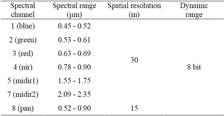
Table 2. 7 Spectral bands of ETM+ (Reflective).
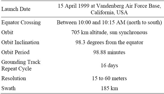
Table 3. Sensor/platform characteristics: ETM+.
mentation and object-based classification. While we used a multi-resolution segmentation algorithm to transform a discrete image into homogeneous regions whose size was equal or greater than the spatial resolution of the sensor, the fuzzy object rule-based classification was used to assign the class labels. The multi-resolution segmentation algorithm applies the principle of minimizing variability among pixel values contained in the scale parameter selected. Different parameters were tested. The starting parameter was the spatial resolution of the ETM+ sensor which resulted into 166 image objects. Changing the scale parameter to 60 resulted into 153 image objects. The resulting image objects with this parameter were larger compared to the 30 parameter. The following sequence of scale parameters was tested: 30, 60, 90, 120, 150, 180, 210 and 240. Figure 2 shows the trend of image objects for the applied scale parameters in that sequence. Apart from the decrease in number of image objects as a result of increase in scale parameter, the total size of the lake changed as well. This implies that seasonal variations in water levels influence the estimation of the lake extent at point in time.
Figure 2 shows that at the pixel level, the lake extent is more uncertain. This is due to limitation of sensor spatial and spectral resolution in space, ambiguity due to the point spread function (PSF) at pixel during the sensor re-
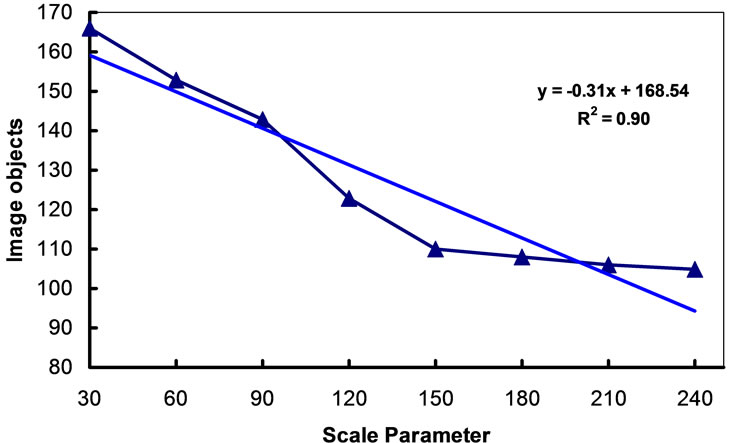
Figure 2. Relationship between scale parameter (level) and image objects.
cording stage and poor definition of lake boundary points [8]. At the pixel level, the pixel values within variability is very high due to atmospheric influence to the electromagnetic energy to and from the Earth’s surface. Sometimes, this can be due to natural scale of occurring. For instance, many shallow lakes and wetlands have discontinuities which are smaller than the sensor spatial resolution that often may result into ambiguity during mapping and monitoring studies.
During experimentation, the scale parameter 150, 180, 210 and 240 yielded small variation in number of image objects. Also these image objects had similar NDVI’s and individual band contribution that help in minimizing uncertainty when classifying. This implies that increasing the sample size results into a decrease in within-variability quantified by standard deviation. Special attention was on the emerging and disappearing image objects at all levels, their spatial locations and size. Figure 3 shows image objects resulting from image segmentation using multi-resolution segmentation algorithm.
2.5. Image Objects Classification
In this case, we used two broad classes, namely, water and non-water. The non-water class comprised of other sub-classes such as wetland, floating vegetation, open shore and shrub land. The class labeling process considered the spatial context of each image object, its location and size and the spectral indices such as NDVI and the band contribution based on the intended application of the respective band. Secondly, the uncertainty for each image object was calculated. Due to sensor limitation in spectral resolution, atmospheric influence on the reflectance, and indeterminate nature of the boundary points of the lake at a point in time, many objects were classified as water. Therefore we exported all image objects classified image objects into Quantum GIS software in which the spatial context for each object was visualized. Since the resulting image objects had various attributes such as NDVI and individual band contribution (band ratio), and
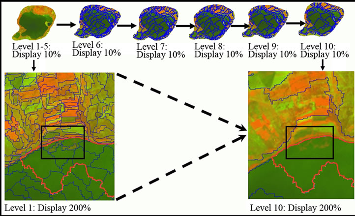
Figure 3. Image objects resulting from image segmentation using multi-resolution segmentation algorithm.
the response of water to all bands is known, it was easier to identify water objects that constituted the lake area. The following condition was used to detect water objects that constituted the lake area:
SELECT water objects
FROM dd/mm/yyyy classified image
WHERE NDVI < 0(3)
Part A of Figure 4 shows sample image objects classified as water and part B of the same figure shows water objects constituting the lake area after applying Equation (3).
2.6. Image Objects with Uncertainty
Through multi-resolution segmentation in Definiens Developer software [9], similar pixels were grouped together into homogeneous image segments corresponding to part of lake area. The size of the resulting segments is governed by the scale parameter while the similarity of pixels is determined by the standard deviation of pixel values from the mean within a given segment. The multiresolution segmentation uses a bottom-up algorithm, which starts at the pixel level and merges the two adjacent segments that give the smallest increase in heterogeneityuntil a heterogeneity threshold is exceeded. The algorithm minimizes locally average heterogeneity of the resulting segments for a given resolution. In our experiment the threshold was based on a combination of spectral values and shape characteristics. Shape was defined by a combination of smoothness and compactness which helped in estimating the irregular shape of the lake area.
Application of different scale parameters (levels) and combinations of spectraland shape characteristics resulted into a hierarchical network of image segments that were topologically linked. Each individual image was segmented at seven levels, characterized with the scale parameter, with the values 30, 60, 90, 150, 180, 210 and 240. The number of image segments decreased with an
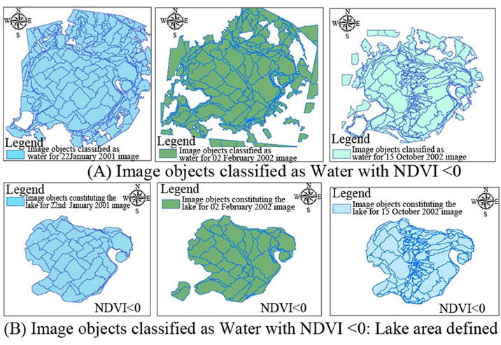
Figure 4. Image objects classification and water objects constituting the lake area tracking using NDVI.
increase in the scale parameter indicating that the spatial extent definition of the lake is parameter sensitive and long term trend analysis is highly affected by seasonal variations in lake levels. Through trial and error process and validating segmentation results with high spatial resolution images on Google Earth we were able to identify the scale at which the spatial extent of the lake at a moment in time could be estimated. Thus at 150 scale parameter, all image segments were automatically merged and the lake area could easily be discriminated from its surroundings. For all images, color, shape and compactness parameters were set at 0.7, 0.2 and 0.8 respectively. To adequately separate water, land, wetlands and floating vegetation, the layer weighting parameters were chosen as 1 for the Near Infrared Radiation (NIR) band and 0.5 for all other bands. Each image segment comprised of a number of attributes such as individual layer mean intensity, image segment brightness, individual layer contribution, NDVI, relative border to adjacent image segments, relative area to defined class that helped in developing rules for classification and uncertainty quantification.
Fuzzy object-based classification was used to label image objects. The classification process was constrained by image objects features such as NDVI, band ratio, adjacency border to another class, etc. Based on the features selected, we determined the degree of membership to a class and quantified it as a percentage. The right hand side of Figure 5 shows the weighted average membership of image objects to lake class. In the same figure, we present the implied spatial uncertainty in lake extent as a result of combination of spatial and temporal scale of measurements as well as the poor definition of the boundary points of the lake in time and space.
Resulting classes were validated by determining the class stability in which the least and the best classified image object of that class were retrieved. Lake area time series were used in linear regression to determine whether there was a trend in lake area.
3. Results
Figure 5 shows the result of the method of mapping the lake as an object with an overall uncertainty over time. The area of the lake shows a shrinking trend for the four years in the study. The uncertainty varies also over time, but as shown in the graph, there is no reason to exclude certain dates from analysis due to indeterminate nature of the lake extent. This approach can be used to analyze large sets of satellite images at different resolution and this will be the best approach towards mapping and monitoring spatial objects over time for change and trend detection. However, the method requires more time during image understanding through image analysis.
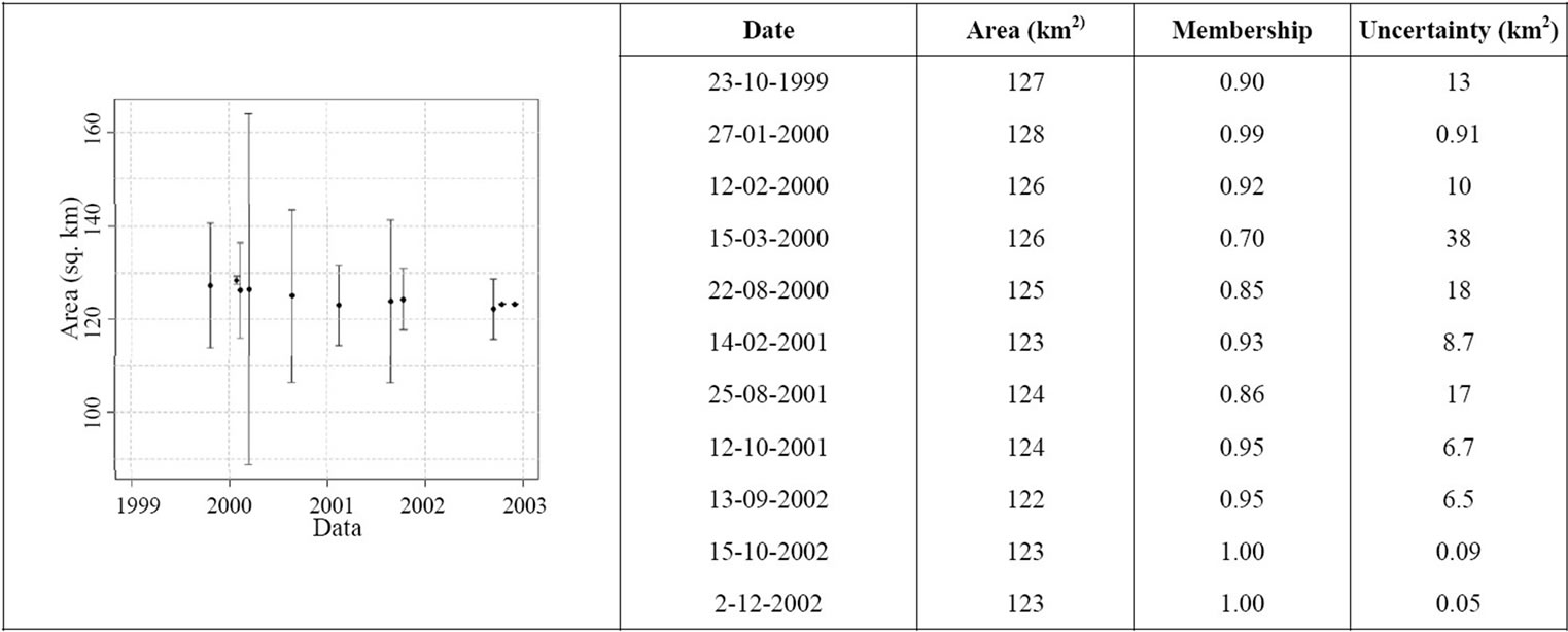
Figure 5. Lake area with uncertainty from 1999 to 2002 from ETM+ images [6].
4. Discussion
The method delineated the lake as an object, while attaching a measure of uncertainty to the entire object. The method gives an overview of trend availability in lake surface area. Trends in lake area can be easily seen and uncertainty of points which are outliers or which have a relatively large influence on the definition of the trend can be checked. Uncertainty in the estimate could also be used to weigh the importance of each estimate in regression, so a more realistic trend line could be obtained. However, the method does not show spatial distribution of uncertainty. It is not clear where the uncertainty is largest, e.g., in the areas with marshes or floating vegetation, or in areas where the image was covered with haze. This method highlights the influence of image quality, as it is easy to see e.g., from Figure 4 for which images of the series the uncertainty in estimated lake surface area is largest.
The method uses a supervised classification algorithm and includes both spectral and spatial characteristics to control the image objects class labeling process. Using the resulting image objects attributes uncertainty in class labeling process is minimized. Therefore the same approach can be adopted in defining the spatial extent of objects with poor definition in space and time.
5. Conclusion and Recommendations
This method provided a viable approach to include uncertainty in mapping and monitoring lake surface area. The method further provides a quick overview and highlights uncertainty related to image quality and time of observation. The same procedure can be adopted in mapping river basins, forest extent and riparian zones. After identification of the surface area we should think of using geospatial approaches in modeling the spatial variability in lake levels.
6. Acknowledgements
The authors express their thanks to Netherlands Fellowship Programme (NFP) for the funds that made this research possible.
REFERENCES
- J. Ijumulana, “Uncertainty in Lake Extent Trends Related to Time and Frequency of Observation,” MSc Thesis, University of Twente, The Netherlands, 2010.
- C. Riungu, “Lake Naivasha Is Dying—Government, Users Wake Up to Nightmare Reality,” Vol. 2010, all Africa.com, 2009.
- S. Mena Lopez, “Papyrus Conservation around Lake Naivasha: Development of Alternative Management Schemes in Kenya,” Enschede, ITC, 2002, p. 87.
- D. M. Harper, K. M. Mavuti and S. M. Muchiri, “Ecology and Management of Lake Naivasha, Kenya, in Relation to Climatic-Change, Alien Species Introductions, and Agricultural-Development,” Environmental Conservation, Vol. 17, No. 4, 1990. p. 328-336. doi:10.1017/S037689290003277X
- A. Hagen, “Fuzzy Set Approach to Assessing Similarity of Categorical Maps,” International Journal of Geographical Information Science, Vol. 17, No. 3, 2003, pp. 235-249.
- A. Stein, N. A. S. Hamm and Y. Qinghua, “Handling Uncertainties in Image Mining for Remote Sensing Studies,” International Journal of Remote Sensing, Vol. 30, No. 20, 2009, pp. 5365-5382.
- P. Fisher, C. Arnot, R. Wadsworth and J. Wellens, “Detecting Change in Vague Interpretations of Landscapes,” Ecological Informatics, Vol. 1, 2006, pp. 163-178. doi:10.1016/j.ecoinf.2006.02.002
- S. Openshaw, “The Modifiable Areal Unit Problem: Concepts and Techniques in Modern Geography 38,” Geobooks, Norwich, 1984.
- “Definiens Imaging, Definiens User Guide [Online],” Accessed on 17 November 2009. http://www.definiens.com/
NOTES
*Corresponding author.