Journal of Geographic Information System
Vol.4 No.2(2012), Article ID:18776,8 pages DOI:10.4236/jgis.2012.42020
Modelling Uncertainty of Stream Networks Derived from Elevation Data Using Two Free Softwares: R and SAGA
1Laboratoire 3E, Ecole Nationale des Ingénieurs de Sfax, Sfax, Tunisia
2Unité de Recherche Dynamique des Bassins Sédimentaires, Paléoenvironnements et Structures Géologiques, Département de Géologie, Faculté des Sciences de Tunis, Université Tunis El Manar, Tunis, Tunisie
3Compus de Beaulieu, Université de Rennes, Rennes, France
Email: hammadi.achour@gmail.com
Received December 24, 2011; revised February 3, 2012; accepted February 20, 2012
Keywords: DEM; Stream Network; Uncertainty Modeling; R; SAGA
ABSTRACT
Stream networks are considered important units in many environmental decision making processes. The extraction of streams using digital elevation models (DEMs) presents many advantages. However it is very sensitive to the uncertainty of the elevation datasets used. The main aim of this paper is to implement geostatistical simulations and assess the propagated uncertainty and map the error of location streams. First, point sampled elevations are used to fit a variogram model. Next two hundred DEM realizations are generated using conditional sequential Gaussian simulation; the stream network map is extracted for each of these realizations, and the collection of stream networks is analyzed to quantify the error propagation. At each grid cell, the probability of the occurrence of a stream and the propagated error are estimated. The more probable stream network are delineated and compared with the digital stream network derived from topographic map. The method is illustrated using a small dataset (8742 sampled elevations) for Anaguid Saharan platform. All computations are run in two free softwares: R and SAGA. R is used to fit variogram and to run sequential Gaussian simulation. SAGA is used to extract streams via RSAGA library.
1. Introduction
A digital elevation model (DEM) is a representation of terrain elevation as a function of geographic location [1]. DEMs have been widely applied to efficiently derive topographic attributes used in hydrologic modelling [2], tectono-geomorphology [3,4], Hazard mapping [5,6] and other applications. DEMs, like other spatial data sets, are subject to error [7,8]. Since DEM error can be propagated through GIS operations and affect the quality of final product. Several factors affect the quality of DEMs [9,10]. A significant source of error can be attributed to data collection. The accuracy of source data varies with collection techniques, such us map digitalization, active airborne sensors, photogrammetric method and field surveying. Other sources of error include the interpolation methods for DEM generation and the characteristics of the terrain surface [11,12].
Methods of errors investigation in DEMs have been widely explored [7,13,14]. The simplest methods are based on criteria such as: differences in elevations between adjacent points [15,16]; elevation histogram analyses [17,18]; systematic detection by inspection of anomalous values within a given moving window [9,19,20]. More complex methods introduce remote sensing and/or geostatistical process. [21,22] have investigated the value of Brownian processes in a fractal terrain simulation model for improving DEM accuracy. [23] used semi-variogram and fractal dimension to describe the pattern of systematic errors. [24] developed a method based on principal component analysis (PCA) to locate random errors in DEMs and to extract uncorrelated patterns.
Techniques of error location and visualization have also been considered. [7] have reviewed research in this domain and noted that DEM contour maps could be a useful tool for error observation, with the possibility of detecting gross errors and blunders. The reliability of this method, however, is not proven. Other more sophisticated methods have focused on error visualization by using RGB multi-band shading technique [25]. More recent attention have been paid to DEM interpolation method on elevation and their mathematical derivatives [25-30]. Techniques of DEM error propagation are commonly classified into two main approaches: the analytical and the stochastic approach [31]. In the first case, the propagated error is derived using some mathematical technique such as via a Taylor series expansion; in the second case, the simulation methods involve stochastic approaches such as Monte Carlo simulation.
This article proposes a methodology to assess errors of stream networks extracted of digital elevation models. It uses a small case study to demonstrate how to implement geostatistical simulations and assess the propagated uncertainty and map the error of location streams. Our secondary objective is to promote the geostatistical tools implemented in the open source environnement for computing (R), and geographical analysis tools implemented in the open source GIS (SAGA). To do so, we adopted an R based robust code written by Hengel, [32]. These scripts used in this article are available on-line via www.geomorphometry.org web site and can be adjusted to any similar case study.
2. Methods and Materials
2.1. Error Propagation: The Monte Carlo Approach
Monte Carlo simulation methods have been used by many researchers to evaluate error in GIS data, including [33-35] and have been applied to specifically address DEM uncertainty. For example, [36] applied Monte Carlo simulation techniques to evaluate the impact of DEM error on viewshed analyses. [37] determined that small DEM errors significantly affected floodplain locations. [38] investigated the impact of DEM error on a forest harvesting model. [39] investigated the effect of simulated changes in elevation at different levels of spatial autocorrelation on slope and aspect calculations. [18] simulated error in DEMs to evaluate slope failure prediction. [40] applied Monte Carlo simulation to assess the impact of DEM error on slope, aspect, and drainage basin delineation.
The basis for using the Monte Carlo method in error propagation analysis is that the original data is perturbed repeatedly by the realisation of the modeled error, and the GIS analysis is calculated from the perturbed data set. Finally, statistical summaries are drawn from the stack of analysis results based on the perturbed data sets [35-37, 41]. In practice, the Monte Carlo method in error propagation of stream networks developed in this study can be summarized in four steps.
• Calculate an experimental variogram from the data and fit a variogram model to represent the variability of the input DEM. This step is achieved by using weighted least squares (WLS) algorithm as implemented in the geoR package.
• Generate multiple realizations of the DEM using conditional simulation. The most common technique in geostatistics used to generate equiprobable realizations of a spatial feature is the Sequential Gaussian Simulation [41]. This step is also achieved by using Stochastic Conditional Gaussian Simulations algorithm as implemented in the gstat package.
• Derive stream network for each realization using the “Channel Network” function, which is available also via the command line “ta_channels” SAGA library, and save the temporary result.
• Estimate probability of the occurrence of stream network. To derive a probability of mapping stream, we need to import all gridded maps of stream, then count how many times the model estimated a stream over a certain grid node. The probability of occurrence of detecting stream is simply the average value of stream from m simulations.
The Monte Carlo approach requires a significantly large number of realizations to produce a reliable estimate of the distribution function. The number of realizations m must be sufficiently large to obtain stable results. Theoretically, the accuracy of the Monte Carlo method is proportional to the square root of the number of runs m [42]. As a rule of thumb, we can take 100 simulations as being large enough, and everything below 20 as insufficient [35]. Consequently, the Monte Carlo method is computationally demanding, particularly when the GIS operation takes much computing time [43].
In this case study the analyses were done with 200 simulation runs, which was a compromise to get reasonably reliable simulation results with moderate computation load. Realizations of the DEM error were done by using sequential Gaussian simulation [41], which has been implemented in open source statistical software R’s extension gstat [44]. The simulated DEMs were further processed for pits removal with the method of Planchon and Darboux [45]. The stream networks were delineated form each simulated DEM using the ta_channels library within SAGA. The different iterations were combined to produce a cumulative probability map representing how many times a cell was part of a stream network.
2.2. Software Tools
In this article we use a combination of statistical and geographical computing software to assess propagated error of detecting streams: SAGA1 (System for Automated Geoscientific Analyses) for geographical computing and R2 for statistical computing. Many spatial packages3 have been developed in recent years, which allow R to be also used for spatial analysis. Three important packages that are used in this paper are gstat [44], geoR [46], and maptools [47]. The link between SAGA and R is made via a special link library RSAGA [48]. A similar link is currently being established to access geoprocessing tools of ESRI’s ArcGIS from within R using the RPyGeo package and a Python interface [49]. The RSAGA package provides access to geocomputing and terrain analysis functions of SAGA by running the command line version of SAGA. RSAGA package provides direct access to SAGA functions including a comprehensive set of terrain analysis algorithms for calculating local morphometric properties (e.g. slope, aspect, curvature), hydrographic characteristics (e.g. size, height, and aspect of catchment areas), and other process-related terrain attributes (e.g. topographic wetness index). In addition, RSAGA provides functions for importing and exporting different grid file formats, and tools for preprocessing grids. Even more detailed instructions of R + SAGA integration can be found in [48,50].
3. Case Study
3.1. Data and Study Area
Figure 1 show the data used in this study. This data consists of 8742-point differential GPS (DGPS) survey conducted for Anaguid seismic project (Saharan platform of Tunisia) in 2010 by CGGV Company, with a variable spatial resolution, ranging from 40 m along survey lines to more 240 m between survey lines, and a positional and vertical accuracy less than 2 cm. This data was used initially to generate multiple realizations of DEM, and then extract drainage network of the study site.
The case study was carried out on a DEM of Anaguid located in southern of Tunisia. This DEM has a 30 m grid cell resolution with 341 × 369 dimension and it was interpolated with the ordinary Kriging method (Figure 1(a)). The study area is enclosed between latitudes 31˚58'N and 31˚52'N and longitudes 9˚45'E and 9˚52'E, covering an area of 111.3 km2. Its elevation ranges from 300 to 440 m with an average and a standard deviation of 36.86. This area is specifically suitable as it presents two contrasting landscapes: plains with terraces in the west and dissected plateau with small valleys in the east direction. Geologically, the area under study is occupied essentially by hard carbonate rocks and conglomerates deposited from the upper Cretaceous to the Neogene.
 (a)
(a) (b)
(b)
Figure 1. Datasets used in this study: (a) Digital elevation model; (b) and (c) Distribution of the data in geographical space; (d) The elevation values are approximately normally distributed.
3.2. Error Propagation in Stream Network
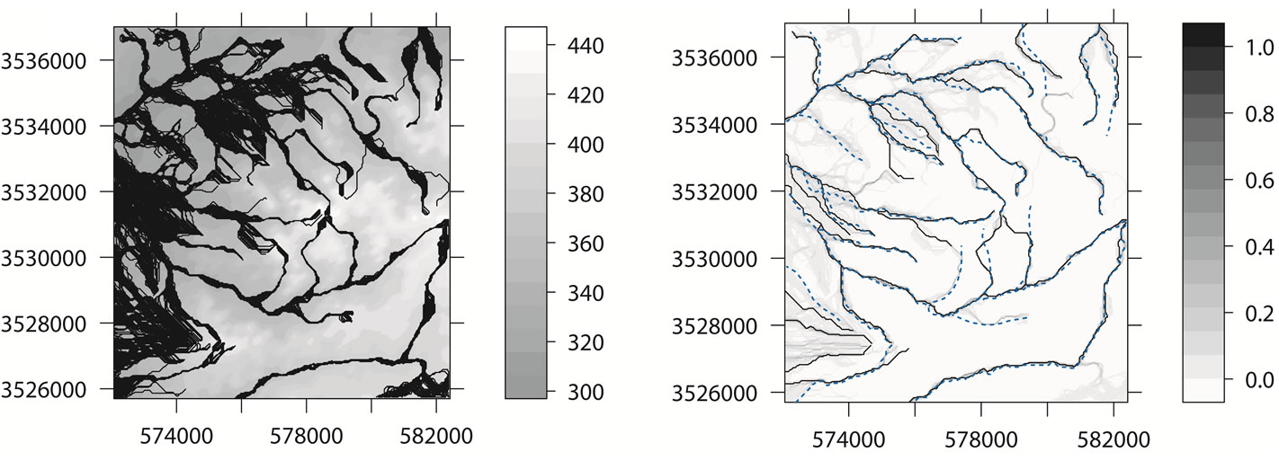
The first results of our analysis are the variograms models fitted using geoR package (Figure 2). These show that the elevation data (Z) in general varies equally in all directions. This is especially distinct for shorter distances which allow us to model the variograms using isotropic models. It is also a relatively smooth variable, there is no nugget variation and spatial autocorrelation is valid (practical range) up to a distance of 2 km. The next results of analysis are the realization of DEMs simulated using Stochastic Conditional Gaussian Simulations algorithm as implemented in the gstat package. To visualize the differences between 200 realizations, we plotted the elevation values of each DEM against their slope values (Figures 3 and 4). In the next step, we look at the dispersion of the stream lines derived for all simulated DEMs. Once the processing is finished, we can visualize all derived streams at top of each other. The spatial distribution of the 200 simulations of stream networks for our study area is shown in Figure 5. The visualization of density of streams clearly illustrates the concept of propagated uncertainty. If you zoom in into this map, you will notice several things. In some areas streams are isolated and hence seem to be very improbable; in other areas stream are densely distributed but over a wider area. Looking at Figure 5(a) we notice that the derived streams show some artificial breaks in the lines. These artifacts are probably a consequence of the fact that we have used arbitrary input parameters for the minimum length of streams (80 pixels) and grid cell size (30 meters). In practice, these parameters should be refined by experts familiar with the study area. In addition, the course of many delineated streams is significantly different in comparison with the streams derived from topographic map as seen in Figure 5(b) which shows clearly the deviations in network delineation. The results from this case study clearly demonstrate the usefulness of the error propagation analysis. By mapping the propagated error we can delineate the most problematic areas and focus our further efforts.
4. Discussion and Conclusions
The delineation of stream networks is important in many environmental and hydrological applications. DEM error propagation can provide valuable additional information for the reliability of stream extraction. The methodology and its application presented here demonstrate an easily employed method to assess DEM error and its impact on stream networks. Previous research used techniques that require higher accuracy data sources such as higher resolution DEMs (LIDAR for example). The reality is that most DEM users do not have such data. The methodology p resented here was designed to remedy this
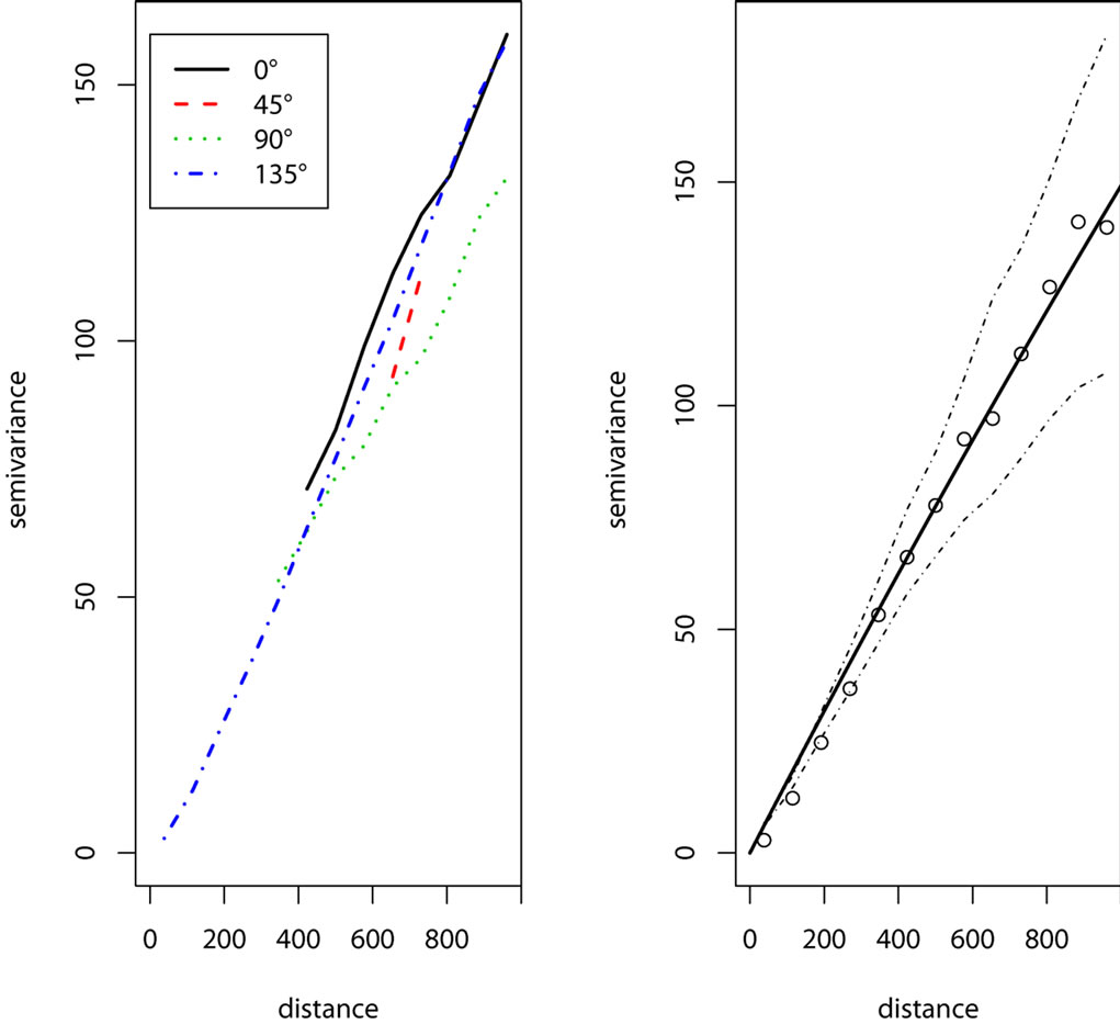
Figure 2. Standard variograms fitted for study area: (left) anisotropy in four directions; (right) isotropic variogram model fitted using the weighted least squares (WLS).

Figure 3. Nine realizations of the DEM following conditional geostatistical simulations. The grayscale legend indicates elevations in meters.
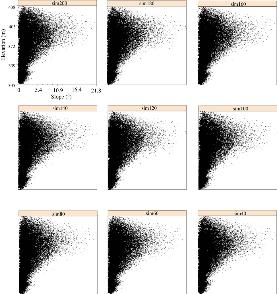
Figure 4. Slope plotted against elevation values for nine DEMs.
 (a) (b)
Figure 5. Uncertainty modelling of stream network derived from elevation data: (a) 200 realizations of stream network overlaid on top of each other. The grayscale legend indicates elevations in meters; (b) Probability of the occurrence of stream networks. The more probable stream network is indicated with black lines. The blue dashed lines indicate digital stream network derived from topographic map.
issue by providing a methodology based on Monte Carlo approach that was successfully implemented using R and SAGA open source software. The purpose of this methodology is to provide DEM users with a suite of tools by which they can evaluate the effect of uncertainty in DEMs and derived topographic parameters. However, some limitations have been identified in this study:
• Firstly, we have limited the number of simulations to 200 runs. It should be feasible to evaluate the increase in accuracy with an increasing number of runs, e.g. by evaluating the change in derived probability or attribute property such as estimated stream length or catchments width. If such a parameter or function does not change anymore below a certain threshold, no more simulations seem to be required.
• Secondly, we have set the grid cell size at 30m without any real justification. It is relevant to evaluate the increase in accuracy with an increasing grid cell size by plotting the error of mapping streams versus the grid spacing index, one can select the grid cell size that shows the maximum information content in the final map. The optimal grid cell size is the one where further refinement does not change the accuracy of derived streams. Future research should aim to perform a more comprehensive evaluation with adaptive cell sizes.
• Thirdly, the computational burden of this method is also an issue. The most costly operations are geostatistical simulations and extraction of stream networks. Geostatistical simulations with standard computer, takes more than 10 minutes to generate 50 simulations for this small study area (341 × 369 pixels). This means that this method is at the moment limited to small data with few hundreds of points; it would be probably of limited use for large data.
• Fourthly, the demonstrated methodology did not assess uncertainty associated with specific DEM applications such as hydrologic modeling or hazard mapping. Researchers can, however, use the uncertainty estimates provided by the proposed simulation techniques to better assess uncertainty for projects that utilize DEMs and DEM-derived data. For example, input parameters for hydrologic models (such USLE) might require elevation and slope values that are frequently obtained directly from a DEM.
• Finally our conclusions are limited to this empirical study of Anaguid with a relatively gentle topography. An obvious future direction is to conduct similar evaluations in other sites with different topographic characteristics to verify the robustness of our results.
5. Acknowledgements
The authors would like to thank the reviewers for their excellent editorial suggestions during the review of this manuscript.
REFERENCES
- T. X. Yue, Z. P. Du, D. J. Song and Y. Gong, “A New Method of Surface Modeling and Its Application to DEM Construction,” Geomorphology, Vol. 91, No. 1-2, 2007, pp. 161-172. doi:10.1016/.02.006
- J. Li and W. S Wong, “Effect of DEM Sources on Hydrologic Applications,” Computers, Environment and Urban Systems, Vol. 34, No. 3, 2010, pp. 251-261. doi:10.1016/j.compenvurbsys.2009.11.002
- G. Peters and R. T. Van Balen, “Tectonic Geomorphology of the Northern Upper Rhine Graben, Germany,” Global and Planetary Change, Vol. 58, No. 1-4, 2007, pp. 310- 334. doi:10.1016/.11.041
- F. Troiani and M. Della Seta, “The Use of the Stream Length-Gradient Index in Morphotectonic Analysis of Small Catchments: A Case Study from Central Italy,” Geomorphology, Vol. 102, No. 1, 2008, pp. 159-168. doi:10.1016/.06.020
- C. J. Van Westen, E. Castellanos and S. L. Kuriakose, “Spatial Data for Landslide Susceptibility, Hazard, and Vulnerability Assessment: An Overview,” Engineering Geology, Vol. 102, No. 3-4, 2008, pp. 112-131. doi:10.1016/.03.010
- R. Nigel and S. D. D. V. Rughooputh, “Soil Erosion Risk Mapping with New Datasets: An Improved Identification and Prioritization of High Erosion Risk Areas,” Catena, Vol. 82, No. 3, 2010, pp. 191-205. doi:10.1016/j.catena.2010.06.005
- P. F. Fisher and N. J. Tate, “Causes and Consequences of Error in Digital Elevation Models,” Progress in Physical Geography, Vol. 30, No. 3, 2006, pp. 467-489. doi:10.1191/0309133306pp492ra
- S. P. Wechsler and C. N. Kroll, “Quantifying DEM Uncertainty and Its Effect on Topographic Parameters,” Photogrammetric Engineering and Remote Sensing, Vol. 72, No. 9, 2006, pp. 108-1090.
- V. Chaplot, F. Darboux, H. Bourennane, S. Leguedois, N. Silvera and K. Phachomphon, “Accuracy of Interpolation Techniques for the Derivation of Digital Elevation Models in Relation to Landform Types and Data Density,” Geomorphology, Vol. 77, No. 1-2, 2006, pp. 126-141. doi:10.1016/j.geomorph.2005.12.010
- C. Chen and T. Yue, “A Method of DEM Construction and Related Error Analysis,” Computers and Geosciences, Vol. 36, No. 6, 2010, pp. 717-725. doi:10.1016/.12.001
- Q. Zhou and X. Liu, “Error Analysis on Grid-Based Slope and Aspect Algorithms,” Photogrammetric Engineering and Remote Sensing, Vol. 70, No. 8, 2004, pp. 957-962. doi:10.1016/.07.005
- L. D. Raaflaub and M. J. Collins, “The Effect of Error in Gridded Digital Elevation Models on the Estimation of Topographic Parameters,” Environmental Modeling and Software, Vol. 21, No. 5, 2006, pp. 710-732. doi:10.1016/.02.003
- J. P. Wilson and J. C. Gallant, “Terrain Analysis: Principles and Applications,” Wiley, New York, 2000.
- S. P. Wechsler, “Perceptions of Digital Elevation Model Uncertainty by DEM Users,” Urban and Regional Information Systems Association Journal, Vol. 15, No. 2, 2003, pp. 57-64.
- M. J. Hannah, “Error Detection and Correction in Digital Terrain Models,” Photogrammetric Engineering and Remote Sensing, Vol. 47, No. 1, 1981, pp. 63-69.
- T. Q. Binh and N. T. Thuy, “Assessment of the Influence of Interpolation Techniques on the Accuracy of Digital Elevation Model,” Journal of Science, Earth Sciences, Vol. 24, No. 4, 2008, pp. 176-183.
- T. Q. Binh and N. T. Thuy, “Assessment of the Influence of Interpolation Techniques on the Accuracy of Digital Elevation Model,” Journal of Science, Earth Sciences, Vol. 24, No. 4, 2008, pp. 176-183.
- K. W. Holmes, O. A. Chadwick and P. C. Kyriakidis, “Error in a USGS 30-Meter Elevation Model and Its Impact on Terrain Modeling,” Journal of Hydrology, Vol. 233, No.1-4, 2000, pp. 154-173. doi:10.1016/S0022-1694(00)00229-8
- A. Felicısimo, “Parametric Statistical Method for Error Detection in Digital Elevation Models,” Journal of Photogrammetry and Remote Sensing, Vol. 49, No. 4, 1994, pp. 29-33. doi:10.1016/0924-2716(94)90044-2
- Q. Zhou and X. Liu, “Analysis of Errors of Derived Slope and Aspect Related to DEM Data Properties,” Computers and Geosciences, Vol. 30, No. 4, 2004, pp. 369-378. doi:10.1016/.07.005
- M. F. Goodchild, “The Fractal Brownian Process as a Terrain Simulation Model,” Modelling and Simulation, Vol. 13, 1982, pp. 1133-1137.
- L. Polidori, “Validation de Modèles Numériques de Terrain, Application à la Cartographie des Risques Géologiques,” Unpublished Doctoral Thesis, Université Paris Diderot, Paris, 1991.
- D. Brown and T. Bara, “Recognition and Reduction of Systematic Error in Elevation and Derivative Surfaces from 7.5-Minute DEMs,” Photogrammetric Engineering and Remote Sensing, Vol. 60, No. 2, 1994, pp. 189-194.
- C. Lopez, “Improving the Elevation Accuracy of Digital Elevation Models: A Comparison of Some Error Detection Procedures,” Transactions in GIS, Vol. 4, No. 1, 2000, pp. 43-64. doi:10.1111/1467-9671.00037
- J. Oksanen, “Tracing the Gross Errors of DEM-Visualization Techniques for Preliminary Quality Analysis,” Proceedings of the 21st International Cartographic Conference, Durban, 10-16 August 2003, pp. 2410-2416.
- J. B. Lindsay and M. G. Evans, “The Influence of Elevation Error on the Morphometrics of Channel Networks Extracted from DEMs and the Implication for Hydrological Modelling,” Hydrological Processes, Vol. 22, No. 11, 2008, pp. 1588-1603. doi:10.1002/.6728
- X. Liu, “Airborne LiDAR for DEM Generation: Some Critical Issues,” Progress in Physical Geography, Vol. 32, No. 1, 2008, pp. 31-49. doi:10.1177/0309133308089496
- I. V. Florinsky, “Accuracy of Local Topographic Variables Derived from Digital Elevation Models,” International Journal of Geographical Information Science, Vol. 12, No. 1, 1998, pp. 47-62. doi:10.1080/136588198242003
- X. Liu and L. Bian, “Accuracy Assessment of DEM Slope Algorithms Related to Spatial Autocorrelation of DEM Errors”. In: Q. Zhou, B. Lees and G. A. Tang, Eds., Advances in Digital Terrain Analysis: Lecture Notes in Geoinformation and Cartography, Springer, Berlin, 2008, pp 307-322.
- J. Schmidt, I. S. Evans and J. Brinkmann, “Comparison of Polynomial Models for Land Surface Curvature Calculation,” International Journal of Geographical Information Science, Vol. 17, No. 8, 2003, pp. 797-814. doi:10.1080/13658810310001596058
- G. Heuvelink, “Analysing Uncertainty Propagation in GIS: Why Is It Not That Simple,” In: G. Food and P. Atkinson, Eds., Uncertainty in Remote Sensing and GIS, Wiley, Chichester, 2002, pp. 155-165.
- T. Hengl, “A Practical Guide to Geostatistical Mapping,” University of Amsterdam, Amsterdam, 2009.
- D. Lanter and H. Veregin, “A Research Paradigm for Propagating Error in Layer-Based GIS,” Photogrammetric Engineering and Remote Sensing, Vol. 58, No. 6, 1992, pp. 825-833.
- S. Openshaw, M. Charlton and S. Carver, “Error Propagation: A Monte Carlo Simulation,” In: I. Masser and M. Blakemore, Eds., Handling Geography Information: Methodology and Potential Applications, Wiley, New York, 1991, pp. 102-114.
- G. B. M. Heuvelink, P. A. Burrough and H. Leenaers, “Propagation of Errors in Spatial Modelling with GIS,” International Journal of Geographical Information Systems, Vol. 3, No. 3, 1989, pp. 303-322. doi:10.1080/02693798908941518
- P. F. Fisher, “First Experiments in Viewshed Uncertainty: The Accuracy of the Viewshed Area,” Photogrammetric Engineering and Remote Sensing, Vol. 57, No. 10, 1991, pp. 1321-1327.
- J. Lee, P. K. Snyder and P. F. Fisher, “Modeling the Effect of Data Errors on Feature Extraction from Digital Elevation Models,” Photogrammetric Engineering and Remote Sensing, Vol. 58, No. 10, 1992, pp. 1461-1467.
- R. Liu and L. Herrington, “The Effects of Spatial Data Error on Forest Management Decisions,” Proceedings of the GIS Symposium, Vancouver, 1993, pp. 1-8.
- G. J. Hunter and M. F. Goodchild, “Modelling the Uncertainty of Slope and Aspect Estimates Derived from Spatial Databases,” Geographical Analysis, Vol. 29, No.1, 1997, pp. 35-49. doi:10.1111/j.1538-4632.1997.tb00944.x
- J. Oksanen and T. Sarjakoski, “Error Propagation of DEMBased Surface Derivatives,” Computers and Geosciences, Vol. 31, No. 8, 2005, pp. 1015-1027. doi:10.1016/j.cageo.2005.02.014
- P. Goovaerts, “Geostatistics for Natural Resources Evaluation (Applied Geostatistics),” Oxford University Press, New York, 1997.
- A. Temme, G. Heuvelink, J. Schoorl and L. Claessens, “Geostatistical Simulation and Error Propagation in Geomorphometry,” In: T. Hengl and H. I. Reuter, Eds., Geomorphometry: Concepts, Software, Applications, Developments in Soil Science, Elsevier, Berlin, 2008, pp. 121- 140.
- G. B. M. Heuvelink, “Error Propagation in Environmental Modelling with GIS,” Taylor & Francis, London, 1998.
- E. J. Pebesma, “Multivariable Geostatistics in S: The Gstat Package,” Computer and Geosciences, Vol. 30, No.7, 2004, pp. 683-691. doi:10.1016/j.cageo.2004.03.012
- O. Planchon and F. Darboux, “A Fast, Simple and Versatile Algorithm to Fill the Depressions of Digital Elevation Models,” Catena, Vol. 46, No. 2, 2001, pp. 159-176. doi:10.1016/S0341-8162(01)00164-3
- J. P. Ribeiro and P. J. Diggle, “Package ‘geoR’: Analysis of Geostatistical Data,” R Package Version 1.6-35, 2011.
- J. N. Lewin-Koh and R. Bivand, “Package ‘Maptools’: Tools for Reading and Handling Spatial Objects,” R Package Version 0.8-10, 2011.
- A. Brenning, “Package ‘RSAGA’: SAGA Geoprocessing and Terrain Analysis in R,” R Package Version 0.92-2, 2011.
- A. Brenning, “RPyGeo: ArcGIS Geoprocessing in R via Python,” R Package Version 0.9-0, 2011.
- T. Hengl, G. B. M. Heuvelink and E. E. Van Loon, “On the Uncertainty of Stream Network Derived from Elevation Data: The Error Propagation Approach,” Hydrology and Earth Sciences Discussions, Vol. 14, No. 7, 2010, pp. 767-799. doi:10.5194/hessd-7-767-2010
NOTES
1http://saga-gis.org
2http://www.r-project.org
3http://cran.r-project.org