Natural Science
Vol. 5 No. 6 (2013) , Article ID: 33096 , 16 pages DOI:10.4236/ns.2013.56091
Iterative approximate solutions of kinetic equations for reversible enzyme reactions
![]()
Department of Mathematics, University of Leicester, Leicester, UK; sarbazmath@yahoo.com, sk464@le.ac.uk
Copyright © 2013 Sarbaz H. A. Khoshnaw. This is an open access article distributed under the Creative Commons Attribution License, which permits unrestricted use, distribution, and reproduction in any medium, provided the original work is properly cited.
Received 27 March 2013; revised 29 April 2013; accepted 6 May 2013
Keywords: Enzyme Kinetics; Homotopy Perturbation Method; Iteration Method; Michaelis-Menten Kinetics; Quasi-Steady State Approximation
ABSTRACT
We study kinetic models of reversible enzyme reactions and compare two techniques for analytic approximate solutions of the model. Analytic approximate solutions of non-linear reaction equations for reversible enzyme reactions are calculated using the Homotopy Perturbation Method (HPM) and the Simple Iteration Method (SIM). The results of the approximations are similar. The Matlab programs are included in appendices.
1. INTRODUCTION
The variety of chemical reactions in a living organism is carried out by enzymes. It appears that the rate of chemical reactions (both forward and backward) is accelerated by enzymes.
They are essential because many chemical reactions occur without the activity of enzymes. Such reactions are linked withan enzyme’s active site, and they become a product after a series of stages. These stages are known as the enzymatic mechanism. There are two types of mechanisms, single substrate and multiple substrate mechanisms [1-4]. An important branch of enzymology is enzyme kinetics which is used to study the rate of chemical reactions. Differential equations are used to characterize the enzyme kinetics based on some principles of chemical kinetics [5-8].
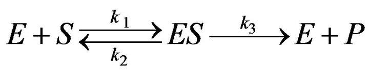
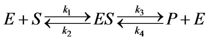
The single enzyme reaction is one of the most powerful kinds of kinetic reaction. Simply put, this enzyme reaction is defined as follows:
 (1)
(1)
where the concentrations of enzyme, substrate, enzymesubstrate complex and product are defined by [E], [S], [ES] and [P], respectively. Also,  and
and  represent the reaction rate constants. By using the idea of mass action, we can describe the reaction Eq.1 in terms of a system of non-linear ordinary differential equations [3].
There are varieties of possible simplifications for the system (Eq.1) to describe analytic approximate solutions of the system. One of the most common approaches to simplify this system is the use of quasi-steady state approxmation (QSSA). The quasi-steady state assumptions occur as fundamental assumptions for enzyme kinetics, and the history of this subject began 80 years ago. It plays a key role with regard to the analysis of the enzyme kinetic equations [5]. Another simplification is the Michaelis-Menten equation created in 1913which pointed that the enzyme reaction (Eq.1) should be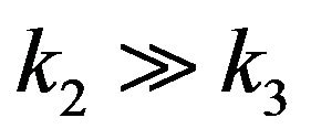 , therefore
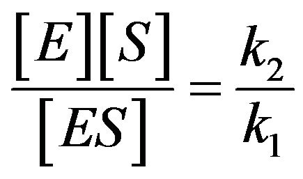 . It means that there is equilibrium between
[E], [S] and [ES] to produce [P] and [E]. In 1925, Briggs and Haldane proposed that the Michaelis-Menten assumption is not always applied. They said that it should be replaced by the assumption that [ES] is present, not necessarily at equilibrium, but in a steady state under condition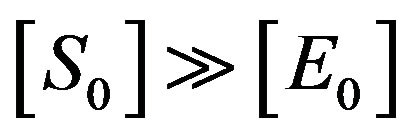 .This means that the concentrations of [ES] occur as a steady state. This is known as the steady state assumption (SSA) or is sometimes called the quasi-steady state approximation (QSSA), or pseudosteady sate approximation [9]. The first description of QSS was given by Briggs and Haldane in 1925 [10]. They described the simplest enzyme reaction in Eq.1, and pointed out the total concentration of enzyme [E], where
 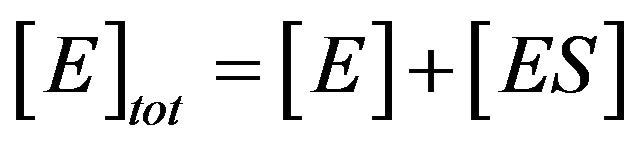 is a tiny value in comparison with the concentration of substrate [S]. Also, they have shown the term of
  is negligible compared to
  and
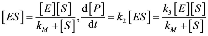
and . As a result, they found the Michaelis-Menten equation, which is a differential equation used to describe the rate of enzymatic reactions. The classical Michaelis-Menten equation is defined as,
 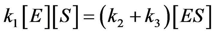 , or
, or
 (2)
(2)
where  is the Michaelis-Menten constant
(for more details see [11]). The purpose of this work is to derive asymptotic approximate expressions for the substrate, product, enzyme and enzyme-substrate concentrations for Eq.3 by using (HPM) and (SIM), and to point out the similarities and differences between the methods of (HPM) and (SIM) for all values of dimensionless reaction diffusion parameters  and
and . Another aim of this project is to find out the appropriate iteration in (SIM) compared to (HPM).
2. MATHEMATICAL FORMULATION
The Michaelis-Menten Eq.1 was applied by Kuhn in 1924 [12] to several cases of enzyme knetics. The model of biochemical reaction was developed by Briggs and Haldane in 1925 [3]. The model of an enzyme action considers a reaction that includes a substrate [S] which binds an enzyme [E] reversibly to asubstrate-enzyme [ES]. The substrate-enzyme leads reversibly to product [P] and enzyme [E]. This mechanism is often written as follows:
 (3)
(3)
The mechanism shows the binding of substrate [S] and the release of product [P] where the free enzyme is [E] and the enzyme-substrate complex is [ES]. In addition,  and
and  denote the rates of reaction. It is clear from Eq.3 that substrate binding and product are reversible. The concentration of the reactants in Eq.3 is denoted by lower case letters:
 (4)
(4)
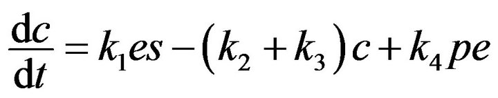
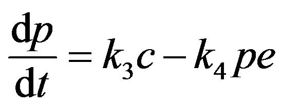
The time of evolution of Eqs.3 and 4 are found by the law of mass action to obtain the set of system of the following non-linear reaction equations:
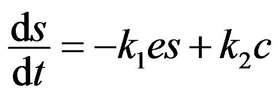 (5)
(5)
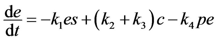 (6)
(6)
 (7)
(7)
 (8)
(8)
when the initial conditions at t = 0 are given by
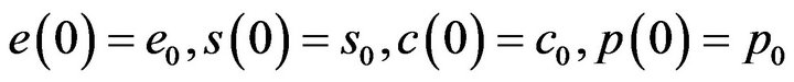 (9)
(9)
Adding Eqs.6 and 7, and using initial conditions Eq.9, we obtain
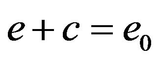 (10)
(10)
Also, adding Eqs.5, 7 and 8, and using initial conditions Eq.9, we get
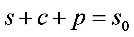 (11)
(11)
By using Eqs.10 and 11, the system of ordinary differential equations (Eqs.5-8) reduce to only two variables, s and c, as follows:
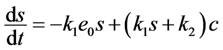 (12)
(12)
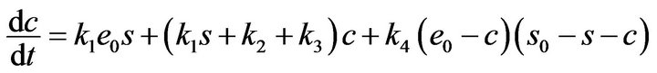 (13)
(13)
with initial conditions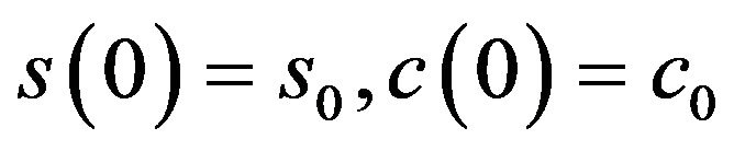 . By introducing the following parameters:
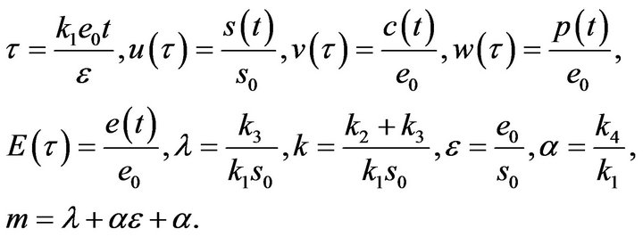 (14)
(14)
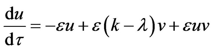
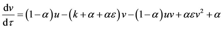
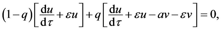
We use the dimensionless technique to reduce the number of parameters for the system of Eqs.12 and 13 and the initial conditions Eq.9. This can be represented in dimensionless form as follows:
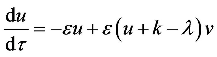 (15)
(15)
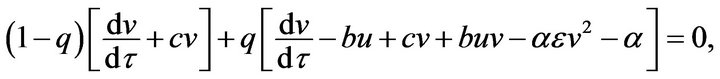
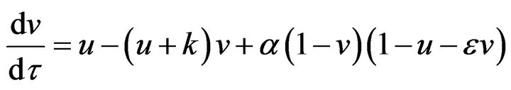 (16)
(16)
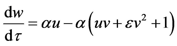 (17)
(17)
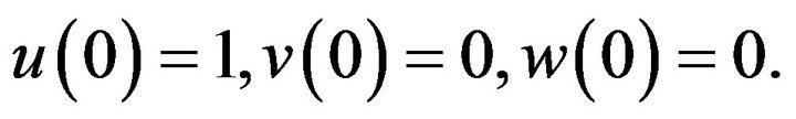 (18)
(18)
In this paper, we estimate the analytic approximate solution for a system of non-linear ODE (Eqs.15-18), by using the methods of (HPM) and (SIM).
3. ANALYTICAL APPROXIMATE SOLUTION USING THE HOMOTOPY PERTURBATION METHOD
The basic idea of the Homotopy-Perturbation Method (HPM) is defined in this section. It is then applied to find the approximate solution of the problem in Eqs.15-18. It is considered from the following function:
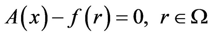 (19)
(19)
with the boundary conditions
 (20)
(20)
where  and
and ![]() are general differential operators, boundary operators, a known analytic function, and the boundary of the domain
are general differential operators, boundary operators, a known analytic function, and the boundary of the domain , respectively [13]. The function
  consists of linear part
 ![]() and nonlinear part N. So, the Eq.19 can be written as:
and nonlinear part N. So, the Eq.19 can be written as:
 (21)
(21)
The Homotopy function is defined by which satisfies
 (22)
(22)
 or
or
 (23)
(23)
where  is an embedding parameter. At the same time,
  is an initial approximation of Eq.19, which satisfies Eq.20. Basically, from Eqs.22 and 23 we can obtain:
 (24)
(24)
 (25)
(25)
Changing  from
from  to
to  depends on the values of
  from zero to unity. It is called deformation in the field of topology. At the same time,
  and
and  are called Homotopy. We use
  as a small parameter initially, and we defined the Eqs.22 and 23 as a power series in
 :
:
 (26)
(26)
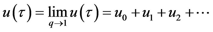
Let  to get the approximate solution of Eq.19
![]() (27)
(27)
Thus, HPM includes a combination of the perturbation method and the Homotopy method. Eqs.15-17 can be solved analytically in a simple and closed form by using the Homotopy Perturbation Method (HPM) (Ref Appendix A). So, the approximate solutions of the system of non-linear differential equations (Eqs.15 and 16) become: (see Eqs.28 and 29).
 (28)
(28)
 (29)
(29)
The analytic expressions of the substrate  and enzyme substrate
  concentrations can be represented in Eqs.28 and 29. The dimensionless concentration of enzyme E can be obtained from Eqs.10 and 14 as follows:
 (30)
(30)
The dimensionless concentration of the product ![]() is obtained either by Eq.17 as follows:
is obtained either by Eq.17 as follows:
 (31)
(31)
or we can use Eqs.11 and 14 to find the concentration of the product ![]() as follows:
as follows:
 . (32)
The simple analytic approximate solution form of the concentrations of enzyme  and product
  for all values of parameters
  and
and , are represented in Eqs.30-32.
4. SIMPLE ITERATION METHOD
In this section, we use a simple technique to find the analytic approximate solution for the system of Eqs.15 and 16. We introduce this method by rewriting Eqs.15 and 16 as follows:
 (33)
(33)
 (34)
(34)
Let 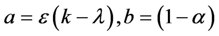 and
and 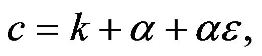 then the Eqs.33 and 34 can be written as:
 (35)
(35)
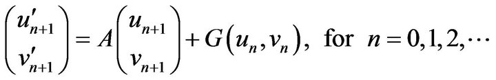
where 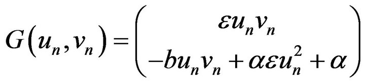 is a non-linear part of the system (Eq.35), and
 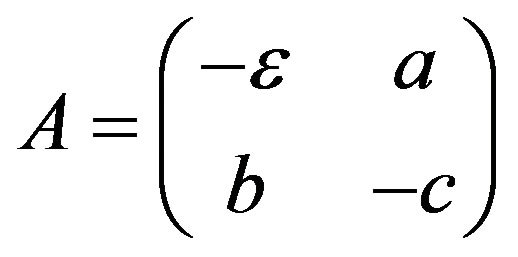 is a matrix of the linear part of the system (Eq.35). To evaluatean approximate solution of Eq.35 with the initial conditions implied by Eq.18, we introduce the following steps to approach the approximate solution.
Step 1. For  and, if possible suppose that
  (just in this step). It means we assume the non-linear part of Eq.35 approaches zero. Consequently, we obtain the following system:
 (36)
(36)
We can solve the system of ordinary differential Eq.36 analytically [14]. So, the solution of Eq.36 with initial conditions (Eq.18) is
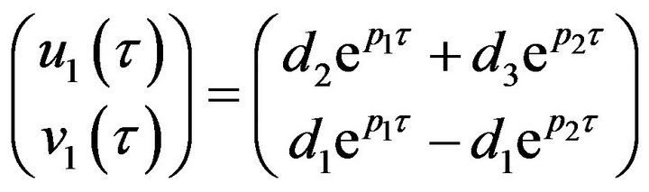 (37)
(37)
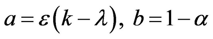
where  and
and  are eigenvalues of matrix A, and
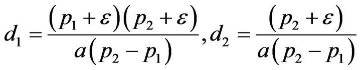 and
and . We substitute
  and
and ![]() in Eq.30 and Eq.32, then obtain
in Eq.30 and Eq.32, then obtain  and
and , respectively. The behaviour of the components in Eq.37 are described in Figures 1-5 (see Appendix C).
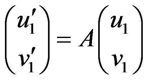
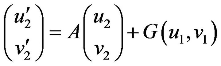
Step 2. For  and substituting Eqs.37 in 35, we obtain the following system of non-linear ODE:
 (38)
(38)
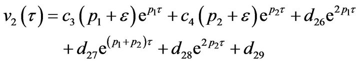
It is clear that the system of non-linear differential equations (Eq.38) is solved analytically [14]. The solution of the system with initial conditions (Eq.18) is obtained as follows:
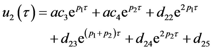 (39)
(39)
 (40)
(40)
where  and
and  are constants. We substitute
  and
and  in Eqs.30 and 32, and obtain
  and
and , respectively. The behaviour of concentrations in this step is described in Figures 6-10 (See Appendix D).
Step 3. For  and substituting Eqs.39 and 40 in Eq.35, we get the following system of non-linear ODE:
 (41)
(41)
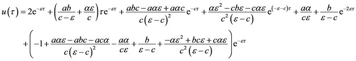
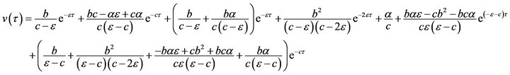
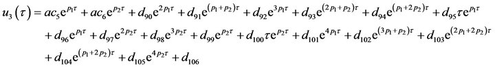
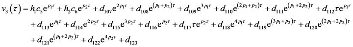
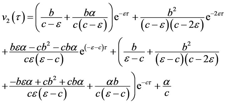
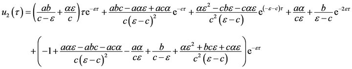
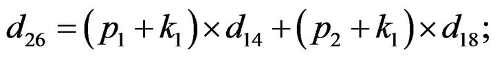
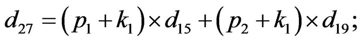
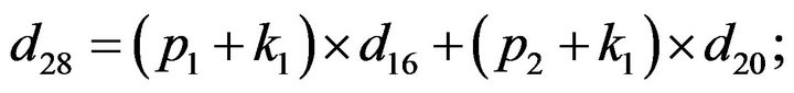
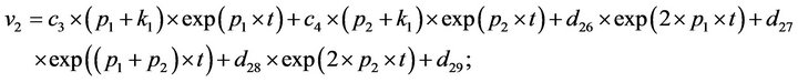
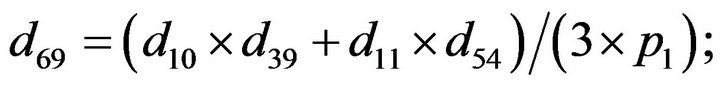
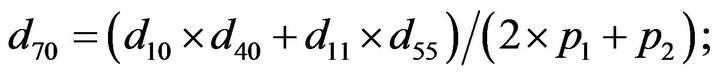
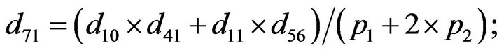
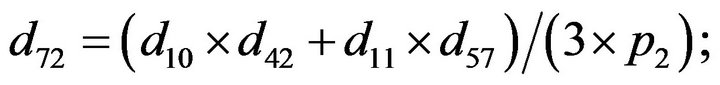
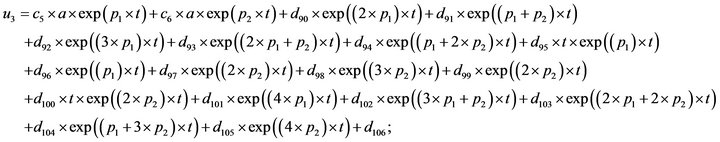
The system of non-linear differential equations (Eq.41) is solved analytically. The solution of the system with initial conditions (Eq.18) is obtained as follows (see Eqs.42 and 43).
Where  and
and  are constants. We substitute
  and
and  in Eq.30 and Eq.32, and obtain
  and
and , respectively. The behaviour of concentrations in this step is described in Figures 11-15 (See Appendix E).
On the other hand, we can easily realize that the behaviour of concentrations u, v, E and w of (HPM) are described in Figures 16-20.
5. ASYMPTOTIC ANALYSIS
An important development of asymptotic analysis was suggested by Kruskal (1963) for differential equations [15]. He defined asymptotology as “the art of describing the behaviour of specified solution (or family of solutions) of a system in limiting case”. The following three different conditions can be identified based on the initial ratio  [16].
[16].
1) If the initial concentration of enzyme  is much greater than the initial concentration of substrate
 (42)
(42)
 (43)
(43)
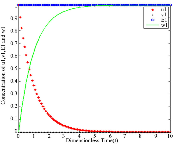
Figure 1. 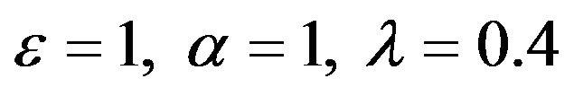 and
and 
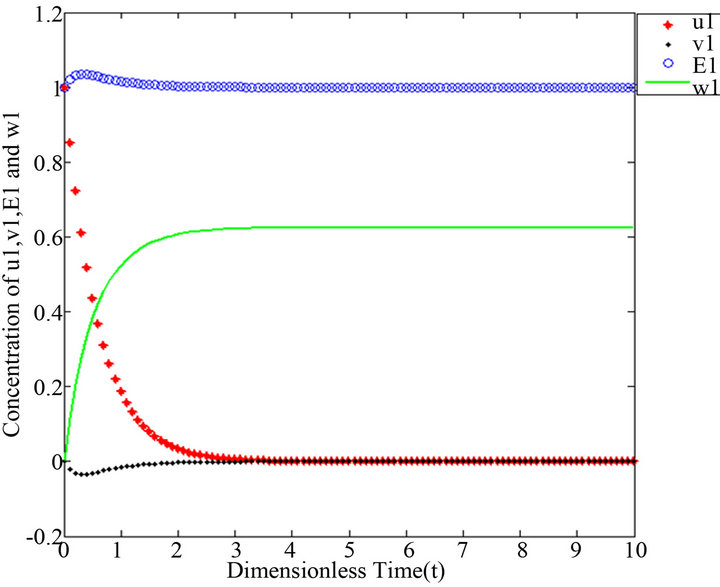
Figure 2.  and
and .
.
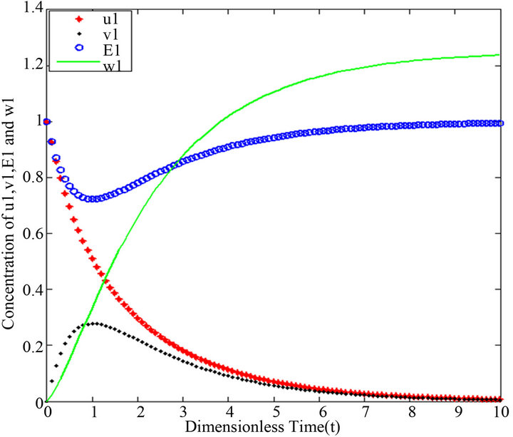
Figure 3.  and
and .
.
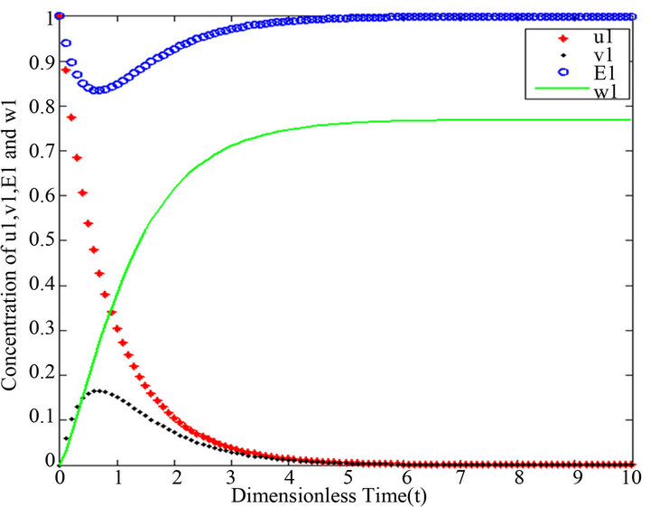
Figure 4.  and
and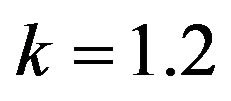 .
.
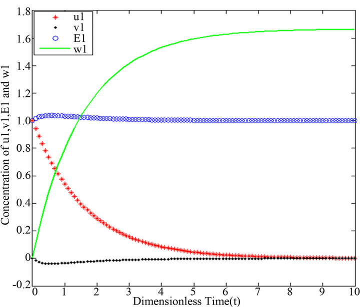
Figure 5.  and
and .
.
Figure 6.  and
and .
.
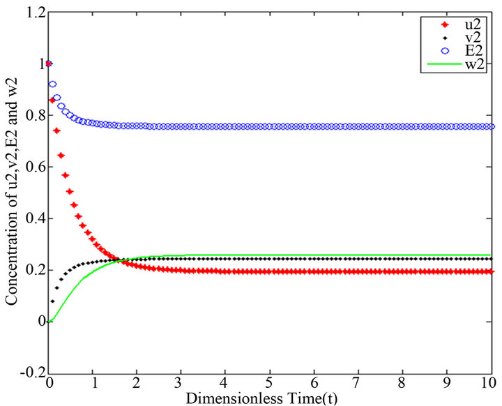
Figure 7.  and
and .
.
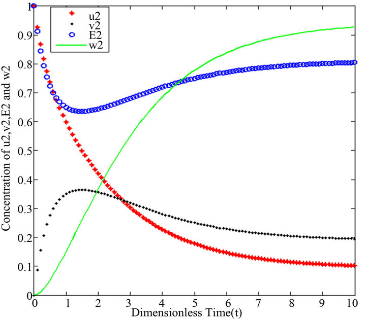
Figure 8.  and
and .
.
 . This means that
 . Also, Schenelland Maini in [2] emphasized that the initial concentration of enzyme greatly exceeds the concentration of substrate, that is
 . So, from Eq.14, we get
 . In this case, the part of the enzyme concentration which binds to the concentration of the substrate is small. This means that there is a free rate of enzyme. This rate is based on the availability of the substrate, and is increased whenever the concentrations of substrate are increased, or by adding additional substrate to the chemical reaction.
2) If the initial concentration of substrate  is much greater than the initial concentration of enzyme
 . This means that
 . So, from Eq.14, we
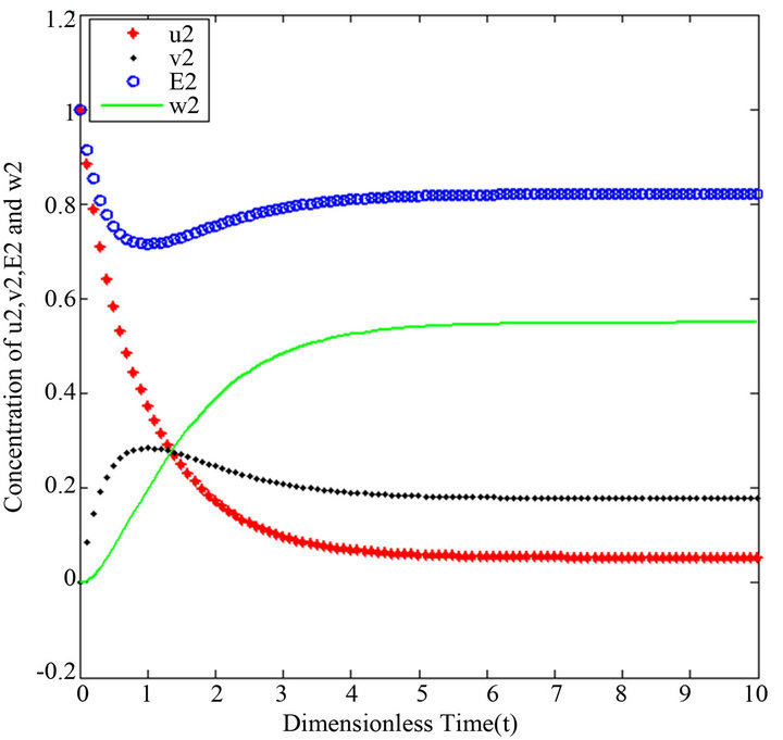
Figure 9.  and
and .
.
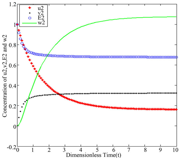
Figure 10.  and
and .
.
obtain . In this case, there is a small part of substrate that links to the enzyme, while a part of it is free. In this case, enzyme molecules usually bind to substrate molecules which mean that a small amount of enzyme is free. The availability of enzyme in this case depends on this rate, and increases when the rate of enzyme is increased, or by adding some extra enzyme to the chemical reaction.
3) If the initial concentration of enzyme and substrate are equal. This means , so from Eq.14, we get
 . In this case, there are no any free molecules of enzyme or substrate. In other words, all substrate molecules are occupied by the enzyme molecules, and all enzyme molecules are also limited by the number molecules of the substrate. Furthermore, if we look the constant rate of reactions
  and
and  from Eq.14, we can define the following conditions:
4) If , then
 .
.
5) If , then
 .
.
6) If , then
 .
.
In addition, according to the definition of ![]() and
and  from Eq.14, we obtain
 , because
  always has a positive value. As result, we can easily combine the Conditions 1-6. We then get the following five basic cases in this paper:
Case 1. The value of  and
and Case 2. The value of
  and
and Case 3. The value of
  and
and Case 4. The value of
  and
and Case 5. The value of
  and
and .
.
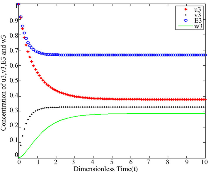
Figure 11.  and
and .
.
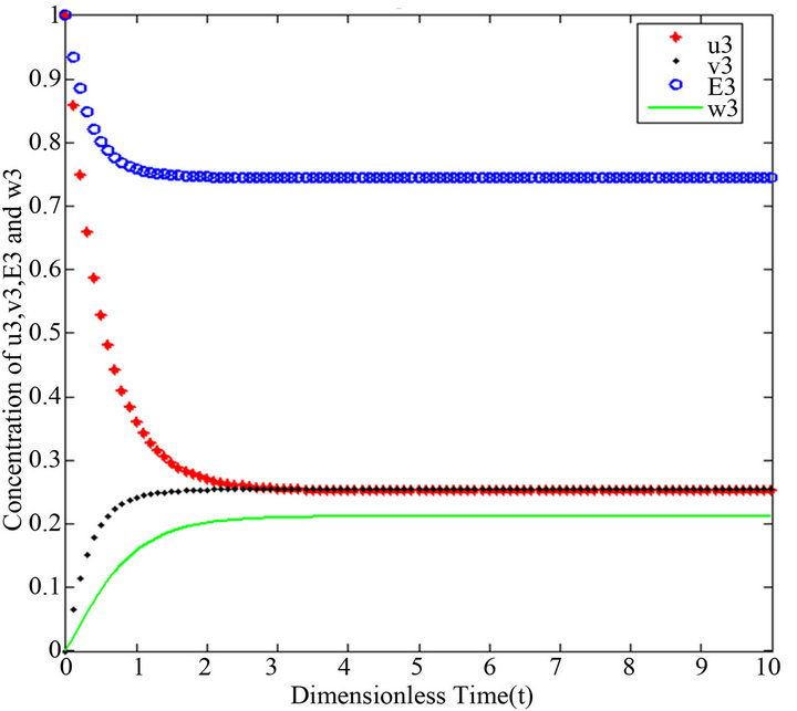
Figure 12.  and
and .
.
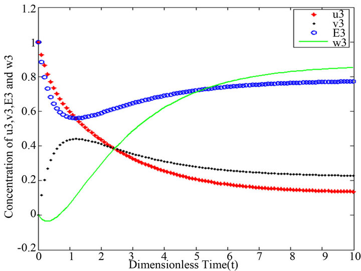
Figure 13. 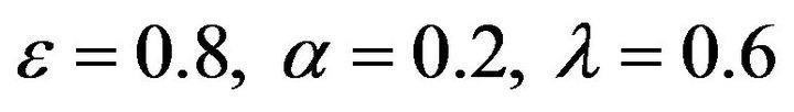 and
and .
.
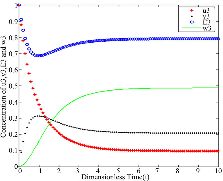
Figure 14.  and
and .
.
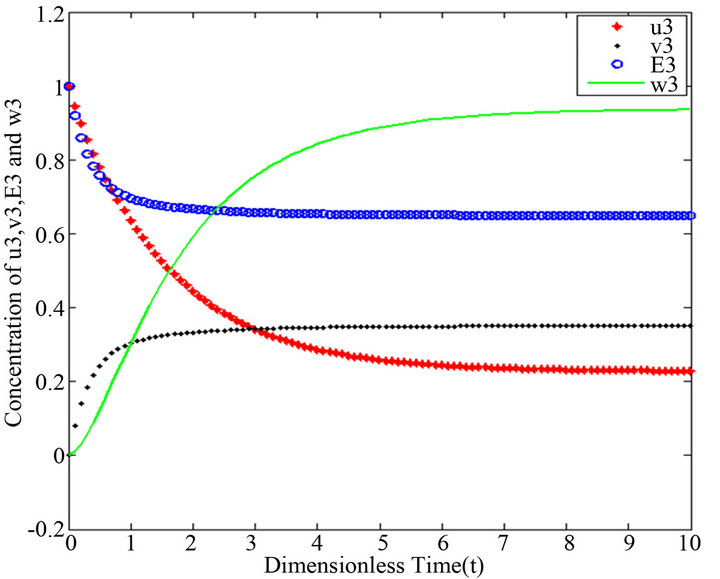
Figure 15.  and
and .
.
We apply the above cases separately in the analytic approximate solution for both methods (HPM) and (SIM).
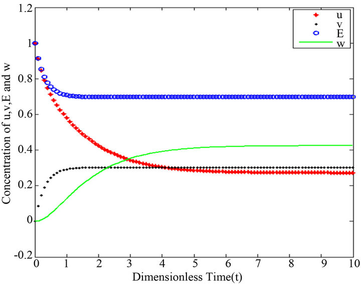
Figure 16.  and
and .
.
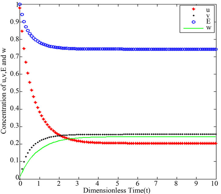
Figure 17.  and
and .
.
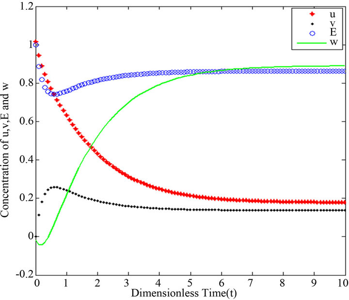
Figure 18.  and
and .
.
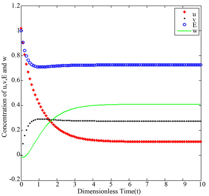
Figure 19.  and
and .
.
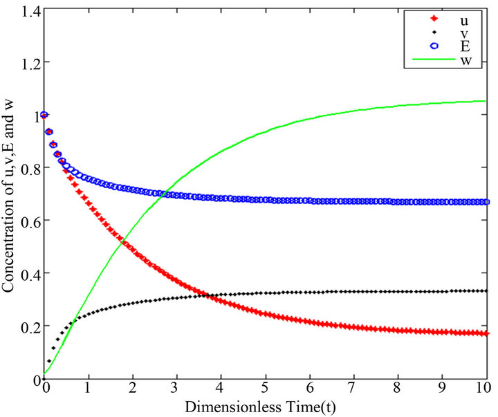
Figure 20.  and
and .
.
6. RESULTS AND DISCUSSIONS
The figures in this section are divided in to four groups. The first three groups are related to three iterations of SIM and the last group refers to the HPM. Figures 1-20 show the analytic approximate solution of substrate![]() , enzyme
, enzyme , enzyme-substrate complex v and product
 . Each figure in this work corresponds to one case in the previous section. The figures change in terms of the values of the dimensionless parameters
  and
and . We have applied two different methods which are SIM and HPM to find the analytical approximate solutions for Eqs.15 and 16. The HPM has been used by many researchers for the system (Eq.1) [1,3,4]. The main purpose of this discussion is to find the similarities and differences between the methods which are used in this study. Another purpose is to recognize the best iteration of the SIM compared to the HPM.
There are a variety of data results that tell us the second iteration in our approach (SIM) is similar to HPM. First of all, the second iteration has many significant similarities compared to (HPM), and some of them provide excellent results in terms of our work. For instance, Figures 6-10 show that the value of the concentration of substrate ![]() slightly decreases from its initial value
slightly decreases from its initial value  and there are a few changes in the value of the concentration of the enzyme-substrate complex v. Generally, they reach some constant values after
 . Also, in Figures 16-20, it appears that the concentration of the components are somewhat similar to those of corresponding Figures 6-10. Another example is that the value of the concentration of enzyme E in both sets of figures is more or less is the same, especially in Cases 1, 2 and 5. Another crucial point is that the value of concentration v in Figure 13 reaches a maximum when
 . Also, in the same interval of time, the value of the concentration v reaches a maximum in Figure 18 as well. We can also realize that the value of the enzyme in both figures ends up at a minimum value when
 . In addition, Figures 11-15 and Figures 16-20 show that there is a gradual decrease in the rate of substrate u between
  which then levels off after
 . On the other hand, the concentration of the product w slightly increases between
  in both set of figures, and is likely to remain stable after
 .
.
However, there are some differences between our simple technique (SIM) and the classical technique (HPM). For example, Figures 1-5 show that the value of the concentration of substrate u slightly decreases from its initial value , and there are a few changes in the value of the concentration of the enzyme-substrate complex v. Generally, they become zero after
 . Meanwhile, in Figures 16-20, it appears that the concentration of the components do not fall to zero, but instead reach some constant values. Basically, it could be pointed out that the differences between them are small and can be therefore be ignored.
Overall, it can be said that the second and third iterations of SIM are appropriate for obtaining a good approximate solution for our case study. In particular, the results of the second iteration are more fitted to an approximate solution in comparison with the classical technique (HPM). However, although there are some different values in terms of results between HPM and the second iteration method, they are tiny.
Figures 1-5. In these profiles of the normalized concentrations of the substrate u, enzyme-substrate complex v, enzyme E and product w correspond to Cases 1-5, respectively. The equations of Step 1 are applied to plot the figures (see Appendix C).
Figures 6-10. In these profiles of the normalized concentrations of the substrate u, enzyme-substrate complex v, enzyme E and product w correspond to Cases 1-5, respectively. The equations of Step 2 are applied to plot the Figures (see Appendix D).
Figures 11-15. In these profiles of the normalized concentrations of the substrate u, enzyme-substrate complex v, enzyme E and product w correspond to Cases 1-5, respectively. The equations of Step 3 are applied to plot the figures (see Appendix E).
Figures 16-20. In these profiles of the normalized concentrations of the substrate u, enzyme-substrate complex v, enzyme E and product w correspond to Cases 1-5, respectively. The Eqs.28 and 32 are applied to plot the figures (see Appendix A).
7. FINDINGS
We have used the mean of the second norm (Eq.44) to find the total differences between the HPM and each iteration of the SIM (see Tables 1-3). The rate of convergence between the SIM and the HPM is shown in Figure 21. Thus, we use the following equation to find this rate of convergence:
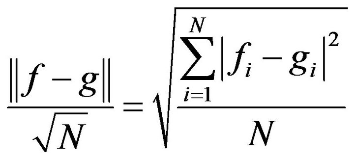 (44)
(44)
where  and
and ![]() are the value of the concentrations of substances u, v, E and w for the SIM and the HPM respectively, and N is the number of timescale iterations. The average norm between the second iteration and HPM is small in value. For instance, the average value of the norm concentration of E is small (equal to 0.02) (see H-S2 in Figure 21). This means that the second iteration method is the most appropriate iteration in this case study in terms of approaching the approximate solution. Although the rate of the second norm for the third iteration is also small (see H-S3), but the second iteration method of our work is the best iteration in order to obtain the convergence in terms of the solution in comparison with the classical method (HPM).
are the value of the concentrations of substances u, v, E and w for the SIM and the HPM respectively, and N is the number of timescale iterations. The average norm between the second iteration and HPM is small in value. For instance, the average value of the norm concentration of E is small (equal to 0.02) (see H-S2 in Figure 21). This means that the second iteration method is the most appropriate iteration in this case study in terms of approaching the approximate solution. Although the rate of the second norm for the third iteration is also small (see H-S3), but the second iteration method of our work is the best iteration in order to obtain the convergence in terms of the solution in comparison with the classical method (HPM).
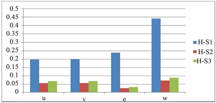
Figure 21. The average value of the second norms convergence between the HPM and the iterations of the SIM.
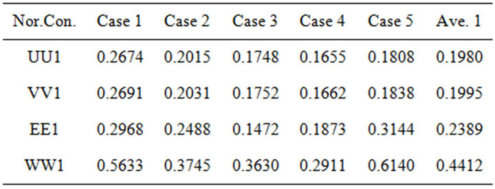
Table 1. The average number of second norms between the first iteration (SIM) and HPM, the results are calculated by using Matlab program (see Appendices B and C).
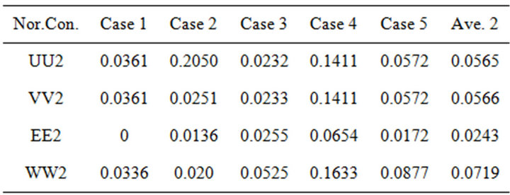
Table 2. The average number of second norms between the second iteration (SIM) and HPM, the results are calculated by using Matlab program (see Appendices B and D).
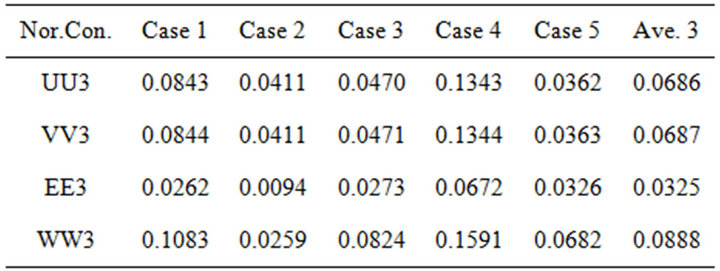
Table 3. The average number of second norms between the third iteration (SIM) and HPM, the results are calculated by using Matlab program (see Appendices B and E).
On the other hand, the differences between our approach (SIM) and the HPM occurred more frequently in the first iteration than in other iterations (see H-S1 values). It could be said that this iteration is not quite appropriate in this case study. This may be caused by giving the non-linear part in this iteration a zero value (see Step 1).
The blue column (H-S1), red column (H-S2) and green column (H-S3) describe the second norm differences between (HPM) and the iterations of (SIM), respectively. The figure is plotted by using the results of Tables 1-3. The second norm differences are represented by u, v, E and w.
8. CONCLUSION
The simple iteration method (SIM) and the Homotopy Perturbation Method (HPM) are used to find approximate analytic solutions to non-linear differential Eqs.15 and 16. Straightforward methods are derived for estimating the concentrations of substrate u, product w, enzyme-substrate complex v and enzyme E. The dimensionless technique applies to reduce the non-linear system of ODE. The HPM was used for a simple enzyme reaction (Eq.1) [1,3]. We have used this method for our case study, and have obtained an analytical approximate solution. Furthermore, a simple approach technique (SIM) was applied. This consisted of three iterations (steps). The approximate solution of the second step is similar to the classical method (HPM) (see Figures 6-10 and Figures 16-20). We have also used the idea of the second norm to determine the best iteration for the problem. So, it is clear that the second iteration method is quite similar to the HPM. Consequently, Figure 21 shows that the second iteration is the appropriate one (see Figure 21 for the H-S2 values). Thus, the SIM technique could be applied to some other complex chemical reactions to find appropriate solutions, and to describe the behaviour of their parameters. For example, it could be applied to many open path ways in terms of biochemical reactions [17]. In addition, we highly recommend applying the simple approach (SIM) to describe the approximate solutions of complex enzyme reactions [18], the reaction mechanism of competitive inhibitions, and the reaction scheme of allosteric inhibitions [19].
REFERENCES
- Maheswari, M.U. and Rajendran, L. (2011) Analytical solution of non-linear enzyme reaction equations arising in mathematical chemistry. Journal of Mathematical Chemistry, 49, 1713-1726. doi:10.1007/s10910-011-9853-0
- Schnell, S. and Maini, P.K. (2000) Enzyme kinetics at high enzyme concentration. Bulletin of Mathematical Biology, 62, 483-499. doi:10.1006/bulm.1999.0163
- Varadharajan, G. and Rajendran, L. (2011) Analytical solutions of system of non-linear differential equations in the single-enzyme, single-substrate reaction with non mechanism-based enzyme inactivation. Applied Mathematics, 2, 1140-1147. doi:10.4236/am.2011.29158
- Varadharajan, G. and Rajendran, L. (2011) Analytical solution of coupled non-linear second order reaction differential equations in enzyme kinetics. Natural Science, 3, 459-465. doi:10.4236/ns.2011.36063
- Li, B., Shen, Y. and Li, B. (2008) Quasi-steady state laws in enzyme kinetics. The Journal of Physical Chemistry A, 112, 2311-2321. doi:10.1021/jp077597q
- Murray, J.D. (1989) Mathematical biology. Springer, Berlin. doi:10.1007/978-3-662-08539-4_5
- Rubinow, S.I. (1975) Introduction to mathematical boilogy. Wiley, New York.
- Segel, L.A. (1980) Mathematical models in molecular and cellular biology. Cambridge University Press, Cambridge.
- Hanson, S.M. and Schnell, S. (2008) Reactant stationary approximation in enzyme kinetics. The Journal of Physical Chemistry A, 112, 8654-8658. doi:10.1021/jp8026226
- Briggs, G.E. and Haldane, J.B.S. (1925) A note on the kinetics of enzyme action. Biochemical Journal, 19, 338- 339.
- Gorban, A.N. and Shahzad, M. (2011) The michaelis-menten-stueckelberg theorem. Entropy, 13, 966-1019.
- Meena, A., Eswari, A. and Rajendran, L. (2010) Mathematical modeling of enzyme kinetics reaction mechanisms and analytical solutions of non-linear reaction equations. Journal of Mathematical Chemistry, 48, 179186. doi:10.1007/s10910-009-9659-5
- He, J.H. (1999) Homotopy perturbation technique. Computer Methods in Applied Mechanics and Engineering, 178, 257-262. doi:10.1016/S0045-7825(99)00018-3
- Dawkins, P. (2007) Differential equations. http://tutorial.math.lamar.edu/terms.aspx
- Gorban, A.N., Radulescu, O. and Zinvyev, A.Y. (2010) Asymptotology of chemical reaction networks. Chemical Engineering Science, 65, 2310-2324. doi:10.1016/j.ces.2009.09.005
- Kargi, F. (2009) Generalized rate equation for singlesubstrate enzyme catalyzed reactions. Biochemical and Biophysical Research Communications, 382, 157-159.
- Flach, E.H. and Schnell, S. (2010) Stability of open pathways. Mathematical Biosciences, 228, 147-152. doi:10.1016/j.mbs.2010.09.002
- Pedersen, M.G., Bersani, A.M., Bersani, E. and Cortese, G. (2008) The total quasi steady-state approximation for complex enzyme reactions. Mathematics and Computers in Simulation, 79, 10101019. doi:10.1016/j.matcom.2008.02.009
- Goeke, Ch.S., Walcher, S. and Zerz, E. (2012) Computing quasi-steady state reductions. Journal of Mathematical Chemistry, 50, 14951513. doi:10.1007/s10910-012-9985-x
- Appendix A. This appendix consists of the solution of Eqs.15 and 16 by using the HPM. Furthermore, this method is used to derive Eqs.28 and 29 from Eqs.15 and 16, let
 and
and ,
,  (45)
(45) (46)
(46)- with initial conditions,
 (47)
(47) - Thus, by using the HPM [1,3,4], the approximate solution of Eqs.45 and 46 are:
 (48)
(48) (49)
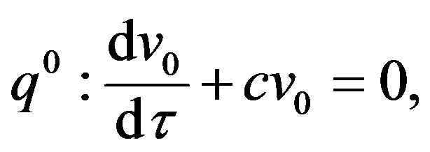
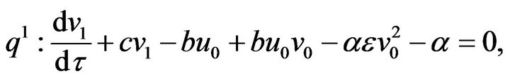
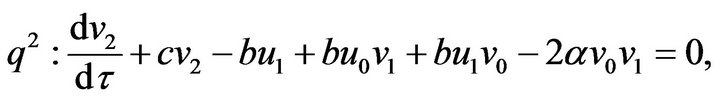
(49)- Substituting the Eqs.48 and 49 in Eqs.45 and 46, and comparing the coefficients of the like power q, we get the following system of ordinary differential equations:
 (50)
(50) (51)
(51)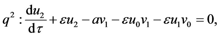 (52)
(52)- and.
 (53)
(53)  (54)
(54) (55)
(55)- The analytical solutions of Eqs.50-55 with initial conditions Eq.47 are:
 (56)
(56) (57)
(57)- and,
 (59)
(59)  (60)
(60) (61)
(61)- According to the HPM, we can easily find that
 (62)
(62)- and,
 (63)
(63) - By putting Eqs.56-58 in Eq.62 and Eqs.59-61 in Eq.63, we obtain the approximate solution for the system of non-linear ODE equations (Eqs.15 and 16) which is described in Eqs.28 and 29.
- Appendix B. Let
 and
and  and we use the following Matlab programming to plot the functions in Eqs.28-32.

 (58)
(58)


- end; plot (T,A,’r’,T,B,’k.’,T,C,’b.’,T,D,’g’) y label (’Concentration of u, v, E and w’) x label (’Dimensionless Time (t)’); axis square.
- Appendix C. Let
 and
and  and we use the following Matlab programming to plot the functions of Step 1.


- plot (T,A,’r’,T,B,’k.’,T,C,’b.’,T,D,’g’) y label (’Concentration of u1, v1, E1 and w1’) x label (’Dimensionless Time (t)’); axis square.
- Appendix D. Let
 and
and  and we use the following Matlab programming to plot the functions in Step 2.


- end; plot (T,A,’r’,T,B,’k.’,T,C,’b.’,T,D,’g’) y label (’Concentration of u2, v2, E2 and w2’) x label (’Dimensionless Time (t)’); axis square.
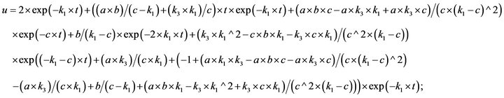
- Appendix E. Let
 and
and  and we use the following Matlab programming to plot the functions in Step 3.


- end; plot (T,A,’r’,T,B,’k.’,T,C,’b.’,T,D,’g’) y label (’Concentration of u3, v3, E3 and w3’) x label (’Dimensionless Time (t)’); axis square.