Engineering
Vol.5 No.5A(2013), Article ID:31870,9 pages DOI:10.4236/eng.2013.55A010
Adaptive Filter for High Dimensional Inverse Engineering Problems: From Theory to Practical Implementation
HOM, SHOM, Toulouse, France
Email: hhoang@shom.fr, remy.baraille@shom.fr
Copyright © 2013 Hong Son Hoang, Rémy Barailles. This is an open access article distributed under the Creative Commons Attribution License, which permits unrestricted use, distribution, and reproduction in any medium, provided the original work is properly cited.
Received February 22, 2013; revised March 23, 2013; accepted April 1, 2013
Keywords: Dynamical Systems; Adaptive Filtering; Stability; Real Schur Decomposition; Stochastic Approximation; Numerical Prediction; Data Assimilation
ABSTRACT
The inverse engineering problems approach is a discipline that is growing very rapidly. The inverse problems we consider here concern the way to determine the state and/or parameters of the physical system of interest using observed measurements. In this context the filtering algorithms constitute a key tool to offer improvements of our knowledge on the system state, its forecast… which are essential, in particular, for oceanographic and meteorologic operational systems. The objective of this paper is to give an overview on how one can design a simple, no time-consuming Reduced-Order Adaptive Filter (ROAF) to solve the inverse engineering problems with high forecasting performance in very high dimensional environment.
1. Introduction
Filtering algorithm constitutes a key tool to offer improvements of system forecast in engineering systems, in particular for oceanographic and meteorologic operational systems. Theoretically, the optimal filtering algorithms provide the best estimate for the system state based on all available observations. As many engineering problems are expressed mathematically by means of a set of partial differential equations together with initial and/or boundary conditions, their numerical solutions result on system state with very high dimension (order of ). In this context the adaptive filter (AF) for state and parameter estimation is an attractive topic for the last decades [1]. Traditionally, the AF is a filter that self-adjusts its parameters (of transfer function) to minimize an error signal. The corresponding nonadaptive filter has then a structure obtained by conventional methods. The AF uses feedback in the form of an error signal to adjust its tuning parameters to optimize the filter performance. It offers an attractive solution to filtering problems in an environment of unknown statistics, provides a significant improvement in performance. AF is successfully applied in many fields as communications, control, noise cancellation, signal prediction, radar, sonar, seismology, biomedical engineering...
One other potential field of application of the AF is numerical weather prediction, in particular, data assimilation. It uses mathematical models of the atmosphere and ocean to predict the weather based on current estimates of weather state [2]. With vast data sets and dimensions of the system state of order , data assimilation requires the most powerful supercomputers in the world. Even though, at the present, for operational purposes we must be satisfied with simplified assimilation methods, not to say on implementation of sophisticated forecast optimal techniques like a Kalman filter (KF) [3] in near future due to requirement on huge memory storage and time evolving the system of equations of dimension
  The difficulties encountered here concern not simply very high dimension of the system state. Factors affecting the accuracy of numerical predictions include the uncertainty in model error statistics, a more fundamental problem lying in the chaotic nature of the partial differential equations used, the density and quality of observations... These difficulties require an another approach to the design of assimilation systems for improving the performance of weather forecasting skills. The objective of this paper is to give an overview of how one can design a simple, no time-consuming Reduced-Order AF (ROAF) with high forecasting performance to handle assimilation problems in the very high dimensional environment.
In the section that follows a brief outline of the theory of ROAF is given. The steps in implementation of the ROAF are detailed in Section 3. Numerical experiments are formulated in Sections 4 and 5 where the problems of estimation of the trajectory of the Lorenz system as well as assimilation of sea surface height (SSH) into the oceanic model are exhibited. Section 6 includes the conclusions.
2. Theoretical Aspects
2.1. Why the Adaptive Filter
The AF, in the context of that designed for estimating the state of very high dimensional system, originates from the work [4] which is defined as a filter minimizing the mean prediction error (MPE) of the system output. One of the main features of the AF is that it is optimal among the members of a set of parametrized state-space innovation representations, with the vector of pertinent parameters of the gain as a control vector. Consider the standard filtering problem
 (1)
(1)
 (2)
(2)
here are uncorrelated sequences of zero mean and timeinvariant covariance
  and
and  respectively. For simplicity, in (2)
 (3)
(3)
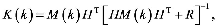
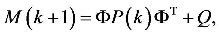
The optimal in mean squared filter is given then by the KF,
 (4a)
(4a)
 (4b)
(4b)
 (4c)
(4c)
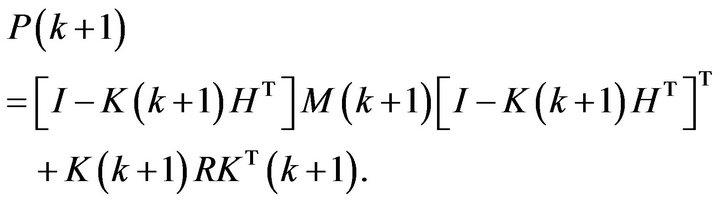 (4d)
(4d)
For systems with a dimension of order  under most favorable conditions (perfect knowledge of all system parameters and noise statistics...) it is impossible to implement the filter (4) in the most powerful computer systems in the world.
In order to exploit the optimal structure of the filter like (4a), noticing that in (4a) all the variables are well defined except the gain . Moreover, under mild conditions, the gain
  will converge to a constant
  [3].
[3].
Thus if instead of all equations in (4) we use only the first equation with assumption that ,
,  is constant, there is an expectation that one can design a filter which is close to the optimal one if
  is close to
  However such asymptotically optimal filter is realizable only if the system dimension is relatively small. To be able to work with any system independently of its dimensionality, in [4] the filter is assumed to be of the form (4) with the gain
  well defined up to the vector of unknown parameters
  Then instead of finding all elements of
 , the task is reduced to seeking an optimal
  of dimension
 , which, as expected, is much less than
 ![]() The best way to carry out this task is to introduce the MPE objective function [4]
The best way to carry out this task is to introduce the MPE objective function [4]
 (5a)
(5a)
 (5b)
(5b)
where  is the mathematical expectation operator,
  denotes the
 ![]() vector norm,
vector norm,  represents a one-step-ahead predictor for
  Mention that the gain in the KF minimizes the objective functions (5a) and (5b) too (under the condition on perfect knowledge of all noise statistics and system parameters...) since
  represents the innovation vector.
Introduction of (5) gives us a great advantage in the design of an ROAF since its minimization can be performed by a simple stochastic approximation (SA) algorithm [5]: At each assimilation instant one has to compute only the gradient of the sample objective function . This makes the task filter design much simpler compared to the KF where the estimation error is minimized in the probability space hence requires the knowledge of probability density functions of all entering random variables. As to Four-Dimensional Variational (4D-Var) [6], the optimization is performed over all assimilation period by iterative algorithms which require, at each assimilation instant, about 20 iterations (each iteration includes one forward model integration and one backward adjoint integration) to approach an optimal control vector. The principal differences between two approaches, 4D-Var and AF, are listed in Table 1.
2.2. Order Reduction and Gain Parameterization
2.2.1. Order Reduction
The ROAF described below has been introduced in [4] in order to reduce the number of estimated parameters in

Table 1. Main differences between 4D-Var and AF.
the gain,
 (6)
(6)
where  projects correction from the reduced space into the full space,
  represents the gain in the reduced space. In [7,8] the choice of
  and parameterization of the gain
  are studied from the point of view of filter stability. It is well known whatever is a filter, the question of ensuring its stability is of the first importance: instability causes the error growth and it can completely destroy the filter. It turns out that under detectability condition, stability of the filter can be guaranteed if the columns of
  is constructed from a subspace of unstable and neutral eigenvectors (EVs) or singular vectors (SVs) of
 . From a computational point of view, it is inadvisable to construct
  from leading eigenvectors or singular vectors: the eigenvectors may be complex, non-orthogonal hence their computation suffers from numerical instability. A great advantage of the singular vector approach is that it does not suffer from numerical instability. There exists the efficient Lanczos algorithm [9] for computing the leading singular vectors of very large sparse systems. However, definition of singular vectors depends on an introduced vector norm and their computation requires the adjoint
  of
of . For many physical problems, the latter represents a very hard task, not to say about the possible existence of discontinuities when obtaining the tangent linear model (TLM)
 .
.
The third approach is related to leading (or dominant) real Schur vectors (ScVs). As proved in [7], the real dominant ScVs (DScVs) play the same role in ensuring filter stability as the dominant EVs or SVs. The Schur approach enjoys all advantages of the singular vector approach and in addition, it does not require the adjoint code. Computation of DScVs is closely associated with searching the direction of rapid growth of the prediction errors (PE). In [10] the PE sampling procedure (SP) based on DScVs is proposed which is aimed at generating the PE samples for the DScVs. These PE samples (will be referred to as DPE (dominant PE) samples) will participate in the construction of  or in the estimation of the parameters of
  to initialize the gain.
2.2.2. Gain Parametrization
In [7] different structures of  are proposed which ensure a stability of the filter (6) if
  is constructed from either dominant EVs or DScVs. For
 (7)
(7)
the symmetric positive definiteness (SPD) of  can guarantee a stability (in
 ![]() norm) of the filter. Thus parameterization of
norm) of the filter. Thus parameterization of  can be made with
  as a vector of tuning parameters provided that
  should be SPD. For adaptation purpose, the following stabilizing gain structure is of more interest due to linear dependence of the gain on the tuning parameters
 (8)
(8)
2.3. Numerical Approximation of 
Generated PE samples share the important property to be iteratively developed in directions of rapid growth of the prediction error. The columns of  constructed from DScVs, allow for capturing the most growing PEs. In [10] the PE sampling procedure is proposed for generating the DScVs samples:
Consider the system (1) at the moment  and let
 —some estimate for the true system state
 — be given. The estimation error is
 . Integration of the model from
  produces the prediction
  at
at . Here
  represents model integration over the interval
 . As the true system state at
  is
is  (for no model error case), the PE
 . Thus integrating
 by the model
  yields the vector
  which can be considered as a PE pattern growing over the period of model integration
 . If we apply this procedure to an ensemble of orthogonal columns
 instead of one vector
the iteration  will produce the sequence
  approaching
 ![]() dominant Schur vectors of
dominant Schur vectors of . The operator
  thus can be approximated by using the columns-vectors of
  which belong to the subspace generated by columns of
 . The filter with the gain constructed on the basis of PE samples will be referred to as a PE filter (PEF).
2.4. Optimization
From a practical point of view, it is often desirable to ensure more than stability for the designed filter. One of the advantages of the AF is that it is self-optimizing, i.e. it is designed to enable self-minimization of the prediction error by tuning the gain parameters. In this sense, the AF can improve its performance that the traditional filters cannot. The objective (5) is based on the deep philosophical idea postulating that the best model should be able to predict the future real process with high precision. As uncertainty in the model always exists, even the KF cannot produce the best estimation in such situation.
From the computational point of view, the choice of the criteria (5) allows us to greatly simplify the optimization procedure. Since the optimality is understood in the mean probabilistic sense, simple optimization tools known as stochastic approximation (SA), and in particular, a simultaneous perturbation SA (SPSA) [5], are quite appropriate for seeking the optimal parameters. With the SPSA, one can compute the gradient vector by additional two times integrating the numerical model. The algorithm is independently on dimension of the vector of tuning parameters. Thus no adjoint equation (AE)  for
for  is needed for the optimization procedure whose construction is a hard task, not to say on the computational time and the cost of integrating AE, possible existence of discontinuities in the numerical model, of non-linearities... For more details, see [11].
3. Practical Implementation of ROAF
The following steps are to be proceeded in order to construct a ROAF.
Step 1. Simulation of an ensemble of DPE samples:
(i) Choice L—a number of DScVs;
(ii) Apply the Sampling Procedure (SP) in [10] to generate an ensemble of PE samples  for L DScVs.
Step 2. Estimation of the filter gain:
(i) Choice of gain structure;
(ii) Estimation of the gain elements from generated PE samples 
(iii) Parametrization of the gain with  as a vector of unknown parameters.
Step 3. Optimization of filter performance: Apply the SPSA algorithm to estimate the tuning parameters . This algorithm is of the form (see [5])
 (9a)
(9a)
 (9b)
(9b)
 (9c)
(9c)
where 
 can be chosen as random variable having the symmetric Bernoulli (+/–) 1 distribution.
For sufficient conditions for convergence of the SPSA iterate  see [5]. In [11] a comparative study on the efficiency of the SPSA with respect to other standard optimization methods shows that the SPSA is more efficient when it is applied to optimizing nonlinear systems and/or when more and more observations are assimilated (the experiment on estimation of the vehicle’s present position and velocity).
Comment 3.1. Due to orthognormalization , the columns of
  are normalized, as a consequence the columns of
  represent only the direction but not the amplitude of PE. For the renormalization procedure, see Comment 2.1 in [10].
Comment 3.2. If at  one assigns
  , the SP generates PE samples using only the numerical model. We have then a so called offline SP (denoted as SP1). In the so-called on-line SP (SP2) the samples are generated during the filtering process. The SP2 simulates the PE by integrating the model from the filtered and its perturbed estimate. The renormalization process can be performed then more precisely if there is a possibility to get some information on the ECM matrix
  of the filtered error
  at
at  assimilation instant (see (4)). For
  -squareroot of
 , the filtered error (FE) sample is obtained from the relation
  The PE patterns in SP2 are generated by integrating the model from
  and
and  at each assimilation instant. They can be used to correct the ECM obtained by the off-line SP1 and to improve the filter performance.
Comment 3.3. For the systems with moderate state dimensions (see the Lorenz system in Section 4), all the elements of the matrix  in (4) can be estimated from the ensemble
 , for example, by
 (10a)
(10a)
 (10b)
(10b)
where  represents a re-normalization factor. For very high dimensional systems, the matrix
  obtained from (10a) is rank deficient. It is therefore advisable to select a well defined structure of the gain with a small number of parameters to be estimated from PE samples. See Section 5 for more details.
4. Experiment on the Lorenz System [10]
The Lorenz attractor is a chaotic map, which shows how the state of a dynamical system evolves over time in a complex, non-repeating pattern [12].
4.1. Problem Statement
The equations that govern the Lorenz attractor are:
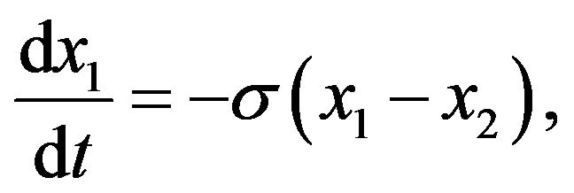 (11a)
(11a)
 (11b)
(11b)
 (11c)
(11c)
where ![]() is called the Prandtl number and
is called the Prandtl number and  is called the Rayleigh number. All
  but usually
  and
and  is varied. The system exhibits chaotic behavior for
  but displays knotted periodic orbits for other values of
 . In the experiments to follow (see also [13]) the parameters
  are chosen to have the values 10, 28 and
  for which the “butterfly” attractor exists.
It is assumed that the observations arrive at the moments  The system (11) is discretized using the Euler method, with the model time step
 . Thus the observations are available after each 200 steps of model integration. The dynamical system corresponding to the transition of the states between two time instants
  and
and  thus can be represented in the form (1) with nonlinear
 . In (1)
  simulates the model error. The sequence
  is assumed to be a white noise having variance 2, 12.13 and 12.13 respectively. As to the observation system, the operator
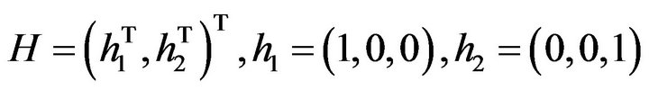 , i.e. the first and third components
  are observed at each time instant
  The noise sequence
  is white with zero mean and variance
  where
where  is unit matrix of dimension
 ![]() The initial estimate in all filters is given by
The initial estimate in all filters is given by  The true system state
  is modeled as the solution of (1) (2) subject to
  added by the Gaussian noise with zero mean and variance 2. The problem considered in this experiment is to apply the PEF and EnKF for estimating the true system state using the observations
  and to compare their performances (see [10] for details).
4.2. The EnKF, PEF and Assimilation
The SP1 has been applied to generate the ensemble of patterns . The pattern
 is obtained at
![]() ,
,  i.e. over the interval equal to that between two observation arrival times. After
 ![]() iterations, the ECM
iterations, the ECM  is estimated using Equations (10a) and (10b) on the basis of
 The gain of the PEF is computed according to the equation for K in (4) subject to the obtained time-invariant M (for a fixed T). According to [14], the gain in the EnKF is updated using the associated Riccati equation and an ensemble of perturbations of the size
  at each assimilation instant
Evolution of the gain element (2,1) in the EnKF subject to  is shown in Figure 1. Mention that for L = 3, L = 30 (not shown here) the variations of the gain in the EnKF are much stronger than for
 . It happens since the perturbations in the EnKF are of random characters. The variation becomes less important with increase in the ensemble size. As reported in [15], the EnKF can yield an accurate performance if the ECM is estimated on the basis of the ensemble of 1000 samples.
The corresponding gain element in the PEF is shown in Figure 1 too. The curves PEF-L1, PEF-L2, PEF-L3 correspond to three simulations subject to 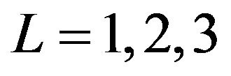 respectively. They are sufficiently smooth after about 20 iterations and behave in a similar way. Generally speaking, the gain element (2,1) in the PEF is greater than that in the EnKF.
Time-average Root-Mean Squrare (RMS) of the FE (RMS-FE), resulting in two filters EnKF and PEF subject to different gains, are presented in Figure 2. In the PEF the gains are time-invariant assuming the values at  (see Figure 1). At the end of the assimilation process, with exception of the EnKF-3, all the filters yield almost the same error level. The RMS of the PE (RMS-PE) produced by the EnKF-3 is too high
 , i.e. being 1.42 times higher than that of the PEF-L1 (with
 ). It is important to stress that due to very slow convergence rate in the MonteCarlo method, the performance of the EnKF can be improved only at an expensive computational cost since the
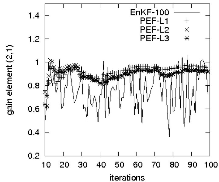
Figure 1. Gain element (2,1) in EnKF-100 and PEFs.
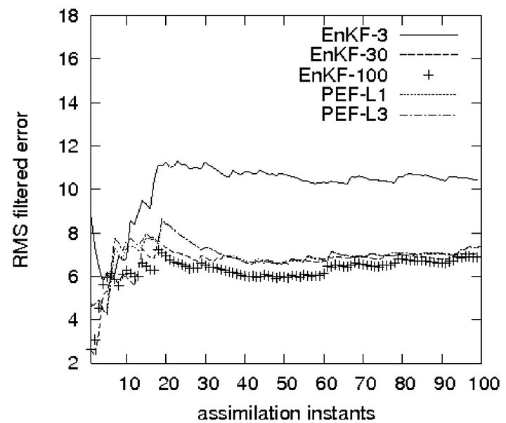
Figure 2. RMS-FE in EnKF and PEF.
ensembles of very large size must be simulated.
In the Lorenz system, for the PEF, the maximal ensemble size (at each time instant) is equal to the dimension of the system state, i.e. equal to 3. Implementation of the EnKF-30 requires, at each assimilation instant, 30 times integration of the numerical model. That is 10 times greater than the dimension of model state. As reported in [15], the EnKF with 19 ensembles produces the estimation error of 3 times higher than that based on 1000 ensembles. In contrast, even with , the performance of the PEF is comparable with that of the EnKF-100.
5. Assimilation in Oceanic Model
5.1. Numerical Model
In this section the ROAF is constructed and applied to assimilate the Sea Surface Height (or topography or relief of the ocean’s surface). The ocean model used here is the Miami Isopycnal Coordinate Ocean Model (MICOM). For the detailed description of the model, see [16]. The model configuration is a domain situated in the North Atlantic from 30.0 N to 60.0 N and 80.0 W to 44.0 W. The grid spacing is about  in longitude and in latitude, requiring Nh = Nx × Ny = 25200 (Nx= 140, Ny = 180) horizontal grid points. The number of layers in the model is
  We note that the state of the model is
  where
where  is the thickness of the lr-th layer,
 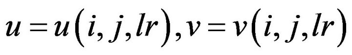 are two meridional and zonal velocity components. The state of the model has the dimension
  In the twin experiments to follow it is assumed that we are given the noise-free observations each
  (days) not at all grid points at the surface but only at the points
5.2. SSH Observations: Reduced-Order Filter
The assimilation problem can be formulated in the form
(1) (2) where  is the system state at
 represents the integration of the nonlinear model over
 ,
,  is the filter gain,
  is the innovation vector. The gain
  has the structure
  The operator
  will interpolate the missing observations from observed points to all horizontal grid points. Symbolically
  is given by
  where
where  are the operators producing correction
  for velocity from layer thickness correction
  using the geostrophy hypothesis. This gain structure can be obtained also by assuming that the covariance
  has the vertical and horizontal separable structure. By considering
  instead of
 , the observation operator can be regarded as
  where
where  is the unit matrix of dimension
  (
( is the number of all horizontal grid points).
5.3. Structure of ECM and Its Estimation
As mentioned in Comment 3.3 (Section 3), the formulas in (10a) and (10b) are appropriate for estimating all the elements of the ECM  only if the system has a moderate dimension (see the Lorenz system in the previous sections). For very high dimensional systems, instead of (10a) and (10b) we introduce the structure
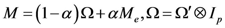 (12a)
(12a)
 (12b)
(12b)
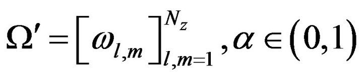
where  denotes the Kronecker product;
  is the number of thickness layers in the model,
  is a scalar representing the covariance of the PE between two layers
  and
and![]() The elements
The elements  can be chosen a priori from physical considerations or estimated from PE patterns. In the well-known Cooper-Haines filter (CHF, see [16,17]), the elements
  are deduced from several physical constraints (conservation of potential vorticity, no motion at the bottom layer...). In the PEF,
  are estimated from DPE patterns. Applying the SP1 subject to
  yields the ensemble of DPE patterns
  from which
  can be estimated through
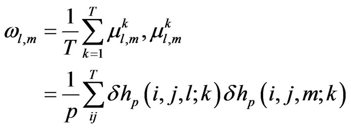 (13)
(13)
where  span all horizontal grid points whose number is equal to
  As the ensemble
  is generated by the model alone, for fixed
  the matrix
  is constant.
In what follows we reserve the notation PEF for the filter subject to ECM (12) with  For
For 
substituting (13) into  (see the gain in (4)) leads to
 .
.
For the present MICOM model,  , the gain in the CHF [2] is equal to
5.4. Parametrization of the Gain. Adaptive Filter
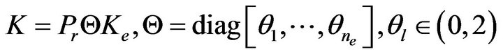
Let  estimated from (13), be decomposed as
  Subject to (6), the gain
  is represented as
  where
where
 with
with  defined as in (7). The adaptive PEF (APEF) is obtained by adjusting
  to minimize (5). The initial values
  correspond to the non-adaptive PEF. For noisy-free observations,
  we have

Figure 3 shows the gain coefficient  in the PEF obtained as functions of iteration
  resulting during application of SP1. Here
 are estimated in accordance
with (13) during application of SP1 subject to  (curve “1L”) and
  (curve “5L”). It is seen that the estimation procedure is robust to the size
 ![]() of sample ensemble.
of sample ensemble.
5.5. Performances of CHF, PEF and APEF
Figure 4 shows the time evolution of the sample objective function  (variances of the SSH innovation) resulting from CHF and PEF.
It is seen that the patterns generated by SP1 allow to well estimate the gain coefficients and as consequence, to improve significantly the performance of PEF compared to that of the CHF: in average, the reduction is of order 50% for the SSH-PE. As to the velocity estimation error, the reduction is of order 40% [11].
The algorithm SPSA (9a)-(9c) has been applied to minimize the objective function (5). Figure 5 shows how the gain component  in the adaptive PEF (APEF) varies during adaptation whereas the gain in the PEF is constant. As expected, self-adjusting the gain parameters allows the APEF to reduce significantly the estimation error that the PEF cannot (see Figure 6).

Figure 3. Estimated gain coefficient .
.
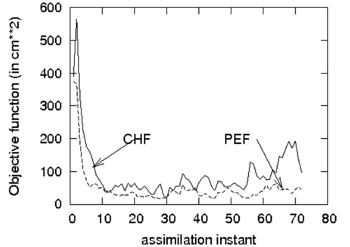
Figure 4. Variances of SSH innovation in CHF and PEF.

Figure 5. Gain in PEF and APEF.
5.6. On-Line SP2
In order to search other opportunities to reduce the estimation errors, the SP2 has been applied along with a re-normalization procedure, without or with the use of Riccati like equation (see Comment 3.2). This allows us to utilize the PE samples generated during assimilation. First we assume that
Here  is obtained from patterns gene-
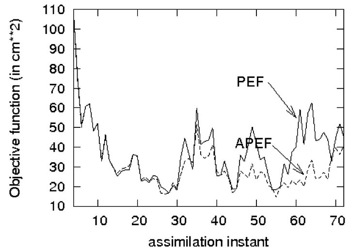
Figure 6. Sample cost functions in PEF and APEF.
rated by SP1 and  is estimated from patterns generated by SP2 during assimilation.
Figure 7 shows SSH PE variances produced by the PEF subject to  (denoted as PEF0) and
  (PEF03). Thus by using PE samples, generated during assimilation, it is possible to extract in addition the information on the prediction error and to obtain a more precise PE covariance matrix and hence to improve the filter performance.
Another way is based on employing a Riccati like equation to estimate the filtered error (FE) patterns. Once having , the ECM of the FE is estimated using the Riccati like equation
Decomposing and following Comment 3.2 one can re-normalize
  as
as
 The ensemble of PE samples
 is generated at the next
  instant and the new
  is estimated from
In Figure 8 the curve “PEF-RIC” represents the SSH PE error produced by the PEF whose gain is updated on the basis of  PE samples simulated at each assimilation instant. It is clear that the “PEF-RIC” behaves better than the “PEF”, especially as assimilation progresses. The price to pay here (compared to PEF) is that one needs to integrate in addition L times the numerical model at each assimilation instant
6. Summary
Theory and practical implementation of the ROAF are presented in this paper. This offers a unified approach to the design of an efficient ROAF with low computational
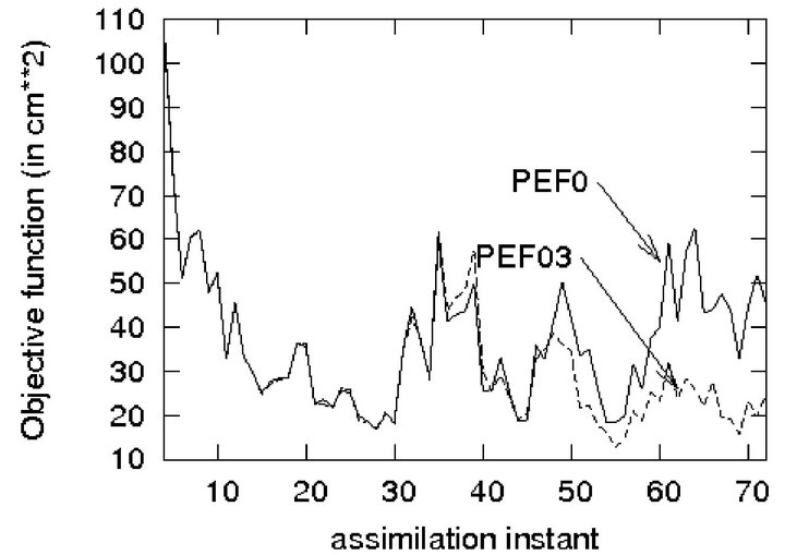
Figure 7. Performance of PEF subject to  and
and  (see (12)).
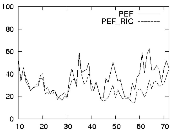
Figure 8. PEF with the gain updated during assimilation by Riccati like equation.
and computer memory cost. It is developed to overcome the difficulties encountered in the filtering problems with very high dimensionality of the system state, uncertainties in the system description, non-linearities... The purpose of this paper is not only to give a comprehensive understanding the basic ideas behind this theory but also intended to provide the potential practitioners a guide for implementation of the ROAF. The ROAF design essentially consists of: 1) Choice of filter gain; 2) Application of a rather simple, but quite powerful PE sampling procedure for generating the PE samples which will participate in the construction of projection subspace and/or initialization of the filter gain; 3) Parametrization of the filter gain and optimization of filter performance by implementing an efficient and low-cost SPSA algorithm which allows to evaluate the gradient of the objective function by 2 times integration of the numerical model.
We mention that compared with traditional optimization methods, the SPSA is proved to be more efficient when working with the non-linear system and/or when more and more observations are assimilated [11]. Due to space limits of this paper we haven’t presented here another important class of filters based on Markovian representation for the PE of system output [18]. This class of filters is proposed by observing that when the designed filter is non-optimal (that is the case in very high dimensional systems) the innovation  does not form an uncorrelated random process and one natural way to improve the filter performance is to include a procedure for whitening the sequence
 . This task can be done efficiently by assuming
  to be a solution of a Markov equation, along with tuning unknown parameters to minimize the variance of the PE system output.
REFERENCES
- S. Haykin, “Adaptive Filter Theory,” Prentice Hall, Upper Saddle River, 2002.
- M. Ghil and P. Manalotte-Rizzoli, “Data Assimilation in Meteorology and Oceanography,” Advances in Geophysics, Vol. 33, 1991, pp. 141-266. doi:10.1016/S0065-2687(08)60442-2
- B. D. O. Anderson and J. B. Moore, “Optimal Filtering,” Prentice-Hall, Inc., Englewood Cliffs, 1979.
- H. S. Hoang, P. De Mey, O. Talagrand and R. Baraille, “A New Reduced-Order Adaptive Filter for State Estimation in High Dimensional Systems,” Automatica, Vol. 33, No. 8, 1997, pp. 1475-1498. doi:10.1016/S0005-1098(97)00069-1
- C. S. Spall, “An Overview of the Simultaneous Perturbation Method for Efficient Optimization, Johns Hopkins APL Technical Digest, Vol. 19, No. 4, 1998, pp. 482-492.
- F. X. Le Dimet and O. Talagrand, “Variational Algorithms for Analysis and Assimilation of Meteorological Observations: Theoretical Aspects,” Tellus, Vol. 37A, 1983, pp. 309-327.
- H. S. Hoang, O. Talagrand and R. Baraille, “On the Design of a Stable Filter for State Estimation in High Dimensional Systems,” Automatica, Vol. 37, No. 8, 2001, pp. 341-359. doi:10.1016/S0005-1098(00)00175-8
- H. S. Hoang, O. Talagrand and R. Baraille, “On the Stability of a Reduced-Order Filter Based on Dominant Singular Value Decomposition of the Systems Dynamics,” Automatica, Vol. 45, No. 10, 2009, pp. 2400-2405. doi:10.1016/j.automatica.2009.06.032
- G. H. Golub and C. F. Van Loan, “Matrix Computations,” 2nd Edition, Johns Hopkins, 1993.
- H. S. Hoang and R. Baraille, “Prediction Error Sampling Procedure Based on Dominant Schur Decomposition. Application to State Estimation in High Dimensional Oceanic Model,” Applied Mathematics and Computation, Vol. 218, No. 7, 2011, pp. 3689-3709. doi:10.1016/j.amc.2011.09.012
- H. S. Hoang and R. Baraille, “On Gain Initialization and Optimization of Reduced-Order Adaptive Filter,” IAENG International Journal of Applied Mathematics, Vol. 42, No. 1, 2011, pp. 19-33.
- E. N. Lorenz, “Deterministic Non-Periodic Flow,” Journal of the Atmospheric Sciences, Vol. 20, No. 2, 1963, pp. 130-141. doi:10.1175/1520-0469(1963)020<0130:DNF>2.0.CO;2
- G. A. Kivman, “Sequential Parameter Estimation for Stochastic Systems,” Nonlinear Processes in Geophysics, Vol. 10, 2003, pp. 253-259. doi:10.5194/npg-10-253-2003
- G. Evensen, “The Ensemble Kalman Filter: Theoretical Formulation and Practical Implementation,” Ocean Dynamics, Vol. 53, No. 4, 2003, pp. 343-367. doi:10.1007/s10236-003-0036-9
- J. T. Ambadan and Y. Tang, “Sigma-Point Kalman Filter Data Assimilation Methods for Strongly Nonlinear Systems,” Journal of the Atmospheric Sciences, Vol. 66, No. 2, 2009, pp. 261-285. doi:10.1175/2008JAS2681.1
- H. S. Hoang, R. Baraille and O. Talagrand, “On an Adaptive Filter for Altimetric Data Assimilation and Its Application to a Primitive Equation Model MICOM,” Tellus, Vol. 57A, No. 2, 2005, pp. 153-170.
- M. Cooper and K. Haines, “Altimetric Assimilation with Water Property Conservation,” Journal of Geophysical Research, Vol. 101, No. C1, 1996, pp. 1059-1077. doi:10.1029/95JC02902
- H. S. Hoang and R. Baraille, “Random Processes with Separable Covariance Functions: Construction of Dynamical Model and Its Application for Simulation and Estimation,” Applied Mathematics & Information Sciences, Vol. 4, No. 6, 2012, pp. 161-171.