Intelligent Control and Automation
Vol.4 No.1(2013), Article ID:27845,10 pages DOI:10.4236/ica.2013.41010
Group Method of Data Handling for Modeling Magnetorheological Dampers
1Department of Electrical Engineering, American University of Sharjah, Sharjah, United Arab Emirates
2Department of Computer Science and Engineering, American University of Sharjah, Sharjah, United Arab Emirates
3Mechatronics Graduate Program, American University of Sharjah, Sharjah, United Arab Emirates
Email: kassaleh@aus.edu, tshanableh@aus.edu
Received October 3, 2012; revised November 15, 2012; accepted November 23, 2012
Keywords: System Identification; Magneto-Rheological Dampers; Group Method of Data Handling; Polynomial Classifier
ABSTRACT
This paper proposes the use of Group Method of Data Handling (GMDH) technique for modeling Magneto-Rheological (MR) dampers in the context of system identification. GMDH is a multilayer network of quadratic neurons that offers an effective solution to modeling non-linear systems. As such, we propose the use of GMDH to approximate the forward and inverse dynamic behaviors of MR dampers. We also introduce two enhanced GMDH-based solutions. Firstly, a two-tier architecture is proposed whereby an enhanced GMD model is generated by the aid of a feedback scheme. Secondly, stepwise regression is used as a feature selection method prior to GMDH modeling. The proposed enhancements to GMDH are found to offer improved prediction results in terms of reducing the root-mean-squared error by around 40%.
1. Introduction
System modeling is instrumental for designing new processes, analyzing existing processes, designing controllers, optimizations, supervision, and fault detection and diagnosis. Nonetheless, it is not always possible to have an explicit mathematical expression for nonlinear systems. Hence, the use of pattern recognition based on input and output patterns of a system is a viable alternative for system identification and modeling [1]. The choice of input patterns, modeling technique, and model architecture are crucial factors in obtaining an accurate model of a system [2]. Various modeling techniques for system identification based on pattern recognition and multivariate regression have been reported in the literature. Artificial neural networks [3], neuro-fuzzy systems [4,5], genetic algorithm [6] and polynomial classifiers [7] are examples of such techniques. In general, these techniques use learning paradigms to estimate the system parameters. As such, the modeling of nonlinear systems of high order entails acquiring large amount of input and output patterns for accurate modeling and identification.
Polynomial classifiers have been used for various applications of classification and regression. It has been shown that they outperform other classical modeling techniques such as neural networks [8].
However, the use of polynomial classifiers becomes prohibitive from computational and storage standpoints when modeling a highly nonlinear systems. Moreover, numerical instabilities may arise due to the need of high order polynomials. Subsequently, the technique of Group Method of Data Handling (GMDH) was introduced [9]. GMDH is a multilayered network of second-order polynomials structured based on a training scenario [10].
In this paper, a variety of GMDH-based techniques are proposed for modeling magnetorheological (MR) dampers and compared against previously published modeling techniques using neural networks and fuzzy logic, and polynomial model [11-13]. An MR damper is filled with a fluid electrically controlled by a magnetic field. The damping characteristics are continuously controlled by varying the power of an electromagnet. MR dampers are semi-active control devices. They have unique characteristics such as low power requirement, fast response rate, mechanical simplicity, low manufacturing and maintenance cost, compactness, and environmental robustness [14]. MR dampers have various applications in many fields such as automotive and biomedical industries. MR dampers possess a highly nonlinear dynamic behavior that is characterized by a system of nonlinear differential equations that cannot be explicitly solved. Hence, as mentioned above, they are often modeled via pattern recognition techniques.
The organization of this paper is as follow. In Section 2 we give an overview of generic system identification and modeling using GMDH. In Section 3 we describe the MR data generation process and propose the use of GMDH for modeling the generated data. Enhanced GMDH-based solutions for MR modeling are proposed in Section 4. Modeling results are discussed and compared in Section 5. Finally, the paper is concluded in Section 6.
2. System Identification with GMDH
GMDH is a modeling technique that provides an effective approach to the identification of higher order nonlinear systems. It was first introduced by A. G. Ivakhnenko [9]. A GMDH is a network comprised of a group of quadratic neurons that are arranged in a special structure to map a given set of training feature vectors into their corresponding response variables. GMDH automatically learns the relations that dominate the system variables during the training process. In other words, the optimal network structure is selected automatically in a way that minimizes the difference between the network output and the desired output. Therefore, GMDH has good generalization ability and can fit the complexity of non-linear systems with a relatively simple and numerically stable network.
GMDH uses a multilayer network of second order polynomials (quadratic neurons) to characterize the complex nonlinear relationships among the given inputs and outputs of a system. Each quadratic neuron has two inputs and a single output. If the two input variables are [x1, x2] the output of each quadratic neuron is calculated as described in Equation (1):
 (1)
(1)
where,  are the weights of the quadratic neuron to be learnt.
Consider a set of training data comprised of N feature vectors each of which is d-dimensional, and a corresponding set of response variables (i.e. targets, {yk; k = 1∙∙∙N}). Accordingly, a GMDH network can be constructed by considering the combinations of all possible input pairs. Each pair of the d dimensions will then be the input to a quadratic neuron of the first layer of the network. Figure 1 shows an example with d = 4; in this case the first layer will be comprised of 6 quadratic neurons. Each neuron will be trained via the well-known least squares method as a second order 2-input polynomial classifier. This training process yields a set of weights for each neuron as shown in Equation (1). For a large number of inputs to any layer, the number of neurons in the subsequent layer can be prohibitively large. As such, a neuron
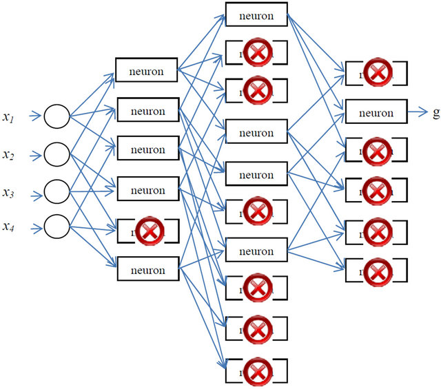
Figure 1. 4-input 3-layer GMDH network example.
selection criterion per layer is required in order to keep the network complexity feasible. More specifically, neuron selection is based on a regularity criterion defined by
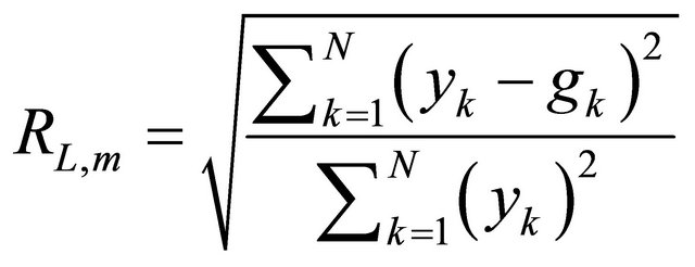 (2)
(2)
where gk is the output of the mth neuron on the Lth layer for the kth feature vector. Consequently, a neuron is selected if its  value is below a certain threshold
 . The threshold is determined based on the maximum and minimum values of
  denoted by
  and
and  respectively such as
 (3)
(3)
where α is a parameter between 0 and 1.
The Lth layer is retained if  is smaller than
 , otherwise, layer number
  would be the last layer in the network (i.e. the output layer). In this layer only the neuron that corresponds to
  is retained. For further illustration, Figure 1 shows an example of the neuron selection process. According to
![]() , only one neuron was eliminated yielding 5 neurons in the first layer. Subsequently, the second layer contains 10 neurons for which
, only one neuron was eliminated yielding 5 neurons in the first layer. Subsequently, the second layer contains 10 neurons for which  is found to be smaller than
 ; hence, layer number 2 is retained. Likewise, according to
 , 4 neurons are retained to comprise the second layer. The third layer contains 6 neurons for which
  is found to be smaller than
  suggesting that this layer will be considered; and according to
  only three neurons will be retained. For the fourth layer
  is found to be larger than
 ; hence this layer is discarded and the neuron corresponding to
  is retained to comprise the output layer.
3. GMDH Application to MR Dampers
3.1. Data Generation
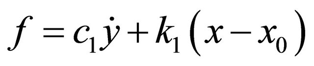
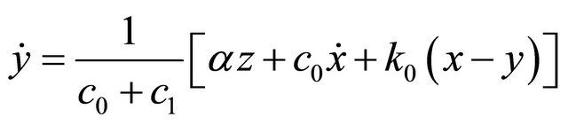
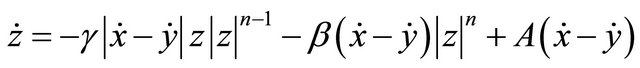
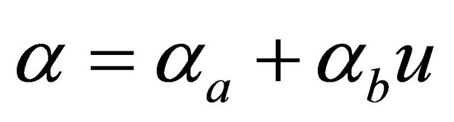
In this work, the mathematical model of the MR damper proposed by Spencer Jr. et al. [15] is used to generate training and testing data that are used in the modeling and evaluation of the proposed GMDH-based solutions. As such, the phenomenological model is governed by the following equations:
 (4)
(4)
 (5)
(5)
 (6)
(6)
 (7)
(7)
 (8)
(8)
 (9)
(9)
 (10)
(10)
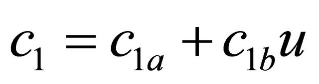
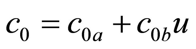
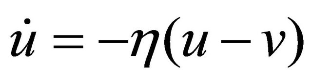
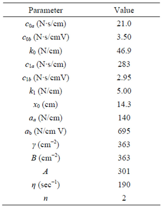
where “x” and “f” are the displacement and the force generated by the MR damper respectively; “y” is the internal displacement of the MR damper; “u” is the output of a first order filter whose input is the commanded voltage, “v”, sent to the current driver. In this model, the accumulator stiffness is represented by k1, the viscous damping observed at large and low velocities are denoted by c0 and c1 respectively; k0 controls the stiffness and large velocities, x0 is the initial displacement of spring k1 associated with the nominal damper force due to the accumulator; γ, β and A are hysteresis parameters for the yield element, and α is the evolutionary coefficient. A set of typical parameters of the 2000 N MR damper is presented in Table 1.
Table 1. 2000 N MR damper parameters [15].
To produce a useful model of an MR damper, the input data must include information in the entire operating range of the system, and cover the spectrum of operation in which the damper functions. Usually, the limits of the input signals are based on the characteristics and applications of the MR damper. Advance knowledge of the input signals enables the generation of a more useful training dataset. The range of the voltage signal is between 0 and 2.5 V. The upper limit (i.e. 2.5 V) represents the saturation voltage of the damper and is obtained experimentally. The saturation voltage implies a voltage level at which no further increase in the yield strength of the damper is exhibited. Similarly, the displacement signal varies within ±2 cm. Matlab is used to generate 4-second worth of simulation data according to equations 4 to 10. This corresponds to 8000 samples, considering that the sampling rate is 2000 Hz. Figure 2 shows the simulated data corresponding to displacement x(n), voltage v(n), and damper force f(n), respectively. The velocity will also be used as an input in modeling the MR damper. Velocity is denoted as s(n) and is obtained by taking the time derivative of the displacement signal.
3.2. Forward Model
In the forward model, the damper force is predicted from the applied voltage. The GMDH has 11 inputs and one single output. The inputs are comprised of three displacement samples, three velocity samples, and three voltage samples taken at times n, n − 1 and n − 2. The remaining inputs are two history samples of the force at times n − 1 and n − 2. The output of the model is the damping force at the current time n, . Out of the generated 8000 data points, 4000 of which are randomly selected for the training set while the remaining 4000 points are used for testing.
After completing the GMDH training, the eleven input variables are reduced to 6 and the irrelevant input variables are automatically eliminated. The relevant inputs of the network are found to be the displacements at times n and n − 2, the voltages at times n and n − 2, and the forces at times n − 1 and n − 2. The final structure of the forward MR damper model is shown in Figure 3.
The prediction accuracy of the GMDH model is evaluated by computing the force root means square error
(RMSE) defined as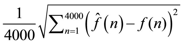 , where
 and
and  are the actual and the predicted forces respectively. The GMDH model described above yielded a force RMSE of 6.44 N. Plots of the time sequences of the predicted and the actual forces along with the prediction error are shown in Figure 4. Plots are shown for the entire time sequence while the RMSE is computed from the testing data only. Figure 4 shows an excellent agree-
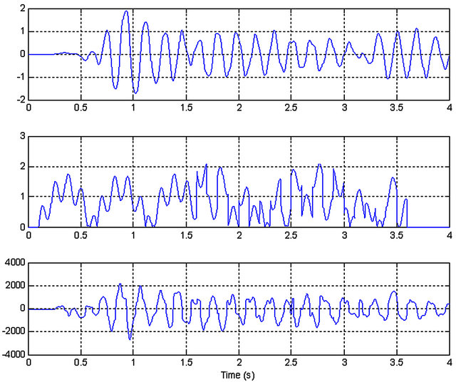
Figure 2. Simulated data for 2000 N MR damper; displacement in cm (top); voltage in volts (middle); and force in Newtons (bottom).
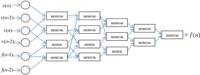
Figure 3. The final structure of forward MR damper GMDH model.
ment between the actual and the predicted force time sequences indicating the adequacy of the GMDH model. The horizontal axis is labeled in seconds where 4 seconds are equivalent to 8000 samples.
3.3. Inverse Model
In the inverse model, the output of the system is the predicted command voltage. To model the inverse MR model, another GMDH network with 11 inputs and one single output is implemented. The inputs to the model are comprised of three displacement samples, three velocity samples, and three voltage samples taken at times n, n − 1 and n − 2. The remaining inputs are two history samples of the voltage at times n − 1 and n − 2.
The output of the model is the command voltage at time n, . After completing the GMDH training, the 11 input variables are reduced to 6, and the rest of the input variables are automatically eliminated. The relevant input variables to the inverse model are shown in Figure 5.
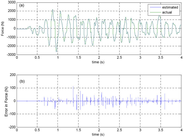
Figure 4. (a) Actual and predicted force using GMDH; (b) Prediction error.
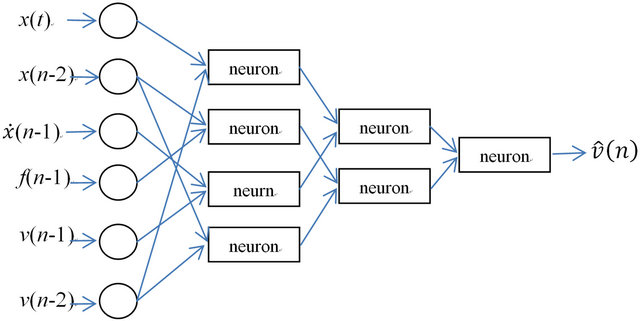
Figure 5. The final GMDH network structure of inverse MR damper model.
The GMDH model of the inverse MR damper yielded a voltage RMSE of 0.03 V. Plots of the time sequences of the predicted and the actual voltages along with the prediction error are shown in Figure 6. Again, plots are shown for the entire time sequence while the RMSE is computed from the testing data only. Like in the forward model, Figure 6 shows an excellent agreement between the actual and the predicted voltage time sequences.
It is worthwhile to mention that we have presented the results in Figures 4 and 6 in the 6th International Symposium on Mechatronics and Its Applications (ISMA’09) [16].
4. Enhanced GMDH Models
While the GMDH models described above resulted in satisfactory prediction results there seems to be further room for improvement to reduce the corresponding RMSE values. As such, two different GMDH-based systems are proposed. In the system, we propose the use of a two-tier architecture in which the estimated force/voltage is augmented to the feature set and the training is carried out again in a second tier. In the second system, we apply the technique of stepwise regression to reduce the dimensionality of feature vectors prior to the evaluation of the
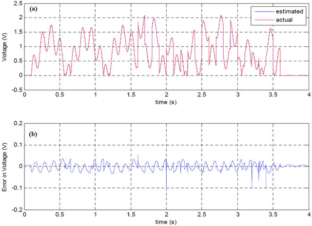
Figure 6. (a) Actual and predicted voltage using GMDH; (b) Prediction error.
GMDH network.
4.1. GMDH with Two-Tier Architecture
The two-tier identification architecture is illustrated in Figure 7. Basically, in the first tier, the training feature vectors and the true Forces or Voltages, depending on whether the forward or backward model is used, are employed to estimate the GMDH network parameters. The network parameters are then used to estimate either the Force or the Voltage of both the training and testing data. In the second tier, the estimated Force or Voltage resulting from evaluating the GMDH network on each vector of the training set is concatenated with that feature vector; hence, adding a new feature variable. Likewise, the estimated Force or Voltage resulting from evaluating the GMDH in on each vector of the testing set is concatenated with that feature vector. The GMDH network is then re-trained using the extended training set. The twotier trained GMDH network is then used to estimate either the Force or the Voltage of the extended testing set.
The prediction results of the force and the voltage of the MR damper using the proposed two-tier approach are shown in Figures 8 and 9 respectively. The reported experimental results show that such architecture noticeably improves the accuracy of the identification process.
4.2. GMDH with Stepwise Regression
In the second proposed system, stepwise regression is
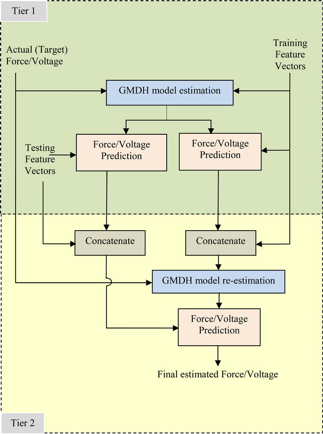
Figure 7. Block diagram of the proposed two-tier system.
used as a preprocessing step to reduce the dimensionality
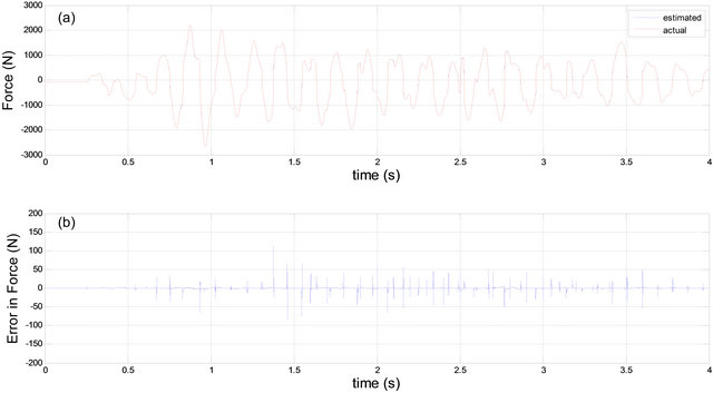
Figure 8. (a) Actual and predicted forces using the proposed two-tier system; (b) Prediction error.
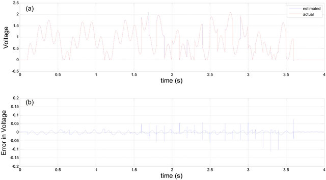
Figure 9. (a) Actual and predicted voltages using the proposed two-tier system; (b) Prediction error.
of the feature vectors [17,18] using the training dataset. The outcome of this step is the indices of the retained dimensions of the feature vectors. This arrangement is further illustrated in the block diagram shown in Figure 10.
Figure 11 shows the prediction results of the force using the stepwise regression with GMDH. Discussing and further comparisons with other methods are given in Section 5.
Alternatively, the stepwise regression procedure can
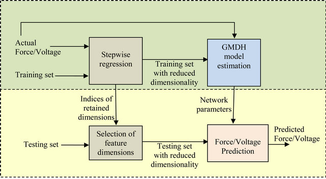
Figure 10. Block diagram of the proposed stepwise regression algorithm with the GMDH.
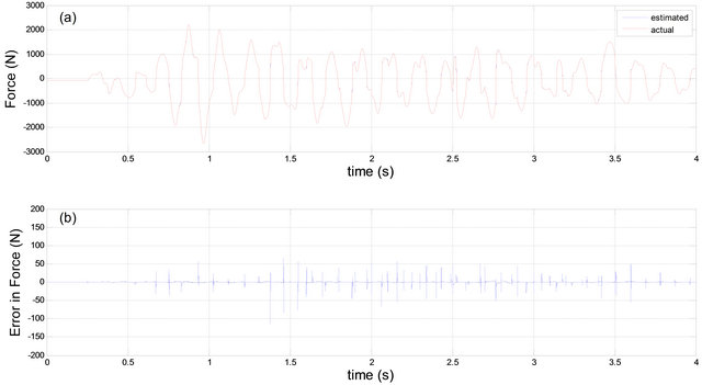
Figure 11. (a) Actual and predicted force using the proposed stepwise regression approach; (b) Prediction error.
be implemented after the polynomial expansion in each neuron in the GMDH network. The stepwise regression procedure is elaborated upon next for completeness.
Stepwise regression is a widely used regressor variable selection procedure. To illustrate the procedure (as described in [16,17]), assume that we have K candidate variables  and a single response variable y. In identification, the candidate variables correspond to the elements of the feature vectors and the response variable corresponds to either the actual force or voltage. Note that with the intercept term β0 we end up with K + 1 variables. In the procedure, the regression weights are iteratively found by adding or removing variables at each step. The procedure starts by building a one variable regression model using the variable that has the highest correlation with the response variable y. This variable will also generate the largest partial F-statistic. In the second step, the remaining K − 1 variables are examined. The variable that generates the maximum partial F-statistic is added to the model provided that the partial F-statistic is larger than the value of the F-random variable for adding a variable to the model, such an F-random variable is referred to as fin. Formally the partial F-statistic for the second variable is computed by:
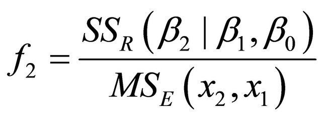 . Where
  denotes the mean square error for the model containing both x1 and x2.
  is the regression sum of squares due to β2 given that β1, β0 are already in the model.
In general the partial F-statistic for variable j is computed by:
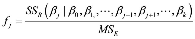 (11)
(11)
If variable x2 is added to the model then the procedure determines whether the variable x1 should be removed. This is determined by computing the F-statistic
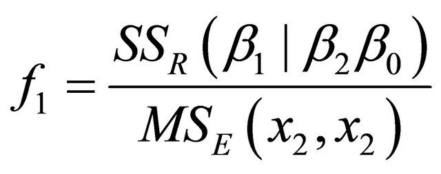 . If f1 is less than the value of the F-random variable for removing variables from the model, such an F-random variable is referred to as fout.
The procedure examines the remaining variables and stops when no other variable can be added or removed from the model. Note that in this work we experiment with a maximum P-value of 0.05 for adding variables and a minimum P-value of 0.1 for removing variables.
Again, note that the elements of the expanded feature vectors are examined using the aforementioned procedure during the training stage of the identification system. The indices of the retained elements of the expanded feature vectors are stored and passed on to the testing or stage. Only the feature vector elements corresponding to the indices found from the training stage are retained.
5. Comparison of Results
In this section we compare the results obtained using the three proposed methods described above (GMDH, twotier GMDH, and GMDH with stepwise regression) with two previously published techniques. These two modeling techniques are neural networks (NN) and adaptive neurofuzzy inference systems (ANFIS) [11,12,19]. The results using ANFIS are taken from [12] since the same dataset has been used in our work. Nonetheless, for NN we have reproduced the results since previous work [11] used a different dataset. The NN architecture that we used is feed-forward network with 11 neurons in the input layer, 22 neurons in the hidden layer and one neuron in the output layer. Network training is done via backpropagation.
The comparison of the prediction results for both force (forward model) and voltage (inverse model) is being done using RMSE values as described above. Figure12 shows the forward model performance (force RMSE values) of the proposed and reviewed methods. Likewise, Figure 13 shows the inverse model (voltage RMSE values) of the proposed and reviewed methods.
Figure 12 indicates that NN is inferior to all other methods while GMDH is superior to ANFIS as it yields a reduction of RMSE by 21%. Furthermore, the two enhanced GMDH techniques outperform ANFIS by approximately 41.7% reduction in the RMSE of the MR damper force prediction.
On the other hand, Figure 13 (inverse model) still indicates that NN is inferior to all other methods while GMDH is comparable to ANFIS. However, only the technique of GMDH with stepwise regression outperforms ANFIS and the two other proposed methods. It is worth mentioning that the GMDH with stepwise regression technique offers a reduction of approximately 40.7% of the RMSE in the MR damper voltage prediction as compared to ANFIS.
Lastly, unlike neural networks and neuro-fuzzy modeling, the proposed GMDH-based techniques can be viewed as layered second order polynomial networks, where the processing function of the node is a polynomial rather than a sigmoid function. Therefore, the optimization in the proposed GMDH-based techniques is based on a series of least-squares fittings rather than iteration-based optimization as in back propagation training of neural networks or ANFIS.

Figure 12. Forward model (force RMSE) of proposed and reviewed methods.
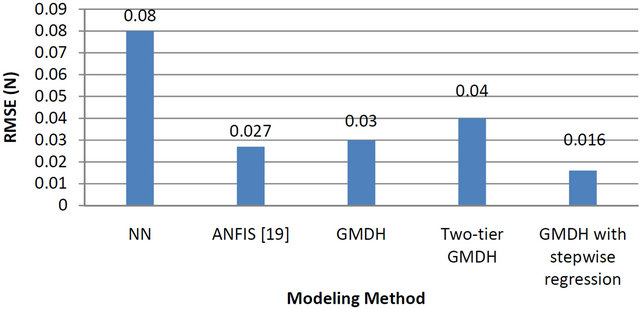
Figure 13. Inverse model (voltage RMSE) of proposed and reviewed methods.
6. Conclusion
In this paper, we investigated the use of GMDH networks for modeling MR200 damper in the context of system identification. We have also introduced two enhanced versions of GMDH networks. Firstly, two-tier architecture was used where the predicted values in the first tier are fed to the network for a second tier training. Secondly, a hybrid of GMDH and stepwise regression in which feature selection is done by stepwise regression prior to GMDH training. Modeling the MR200 damper is done in forward and inverse modes where force and voltages are being predicted respectively. The GMDH-based modeling has been compared to two modeling methods (i.e. NN and ANFIS). GMDH with stepwise regression is found to offer significant reduction of about 40% in RMSE for both forward and inverse models.
REFERENCES
- G. P. Liu, “Nonlinear Identification and Control: A Neural Network Approach,” Springer, New York, 2001. doi:10.1007/978-1-4471-0345-5
- P. R. Water, E. J. H. Kerckhoffs and D. Van Welden, “GMDH-Based Dependency Modeling in the Identification of Dynamic Systems,” European Simulation MultiConference (ESM), 2000, pp. 211-218.
- X. Huang, J. Xu and S. Wang “Nonlinear System Identification with Continuous Piecewise Linear Neural Network,” Neurocomputing, Vol. 77, No. 1, 2011, pp. 167- 177.
- M. Gonzalez-Olvera and Y. Tang, “A New Recurrent Neurofuzzy Network for Identification of Dynamic Systems,” Fuzzy Sets and Systems, Vol. 158, No. 10, 2007, pp. 1023-1035. doi:10.1016/j.fss.2006.10.002
- G. Wang, “Application of Hybrid Genetic Algorithm to System Identification,” Structural Control and Health Monitoring, Vol. 16, No. 2, 2009, pp. 125-153. doi:10.1002/stc.306
- K. Assaleh, “Extraction of Fetal Electrocardiogram Using Adaptive Neuro-Fuzzy Inference Systems,” IEEE Transactions on Biomedical Engineering, Vol. 54, No. 1, 2007, pp. 59-68. doi:10.1109/TBME.2006.883728
- K. Assaleh and H. Al-Nashash, “A Novel Technique for the Extraction of Fetal ECG Using Polynomial Networks,” IEEE Transactions on Biomedical Engineering, Vol. 52, No. 6, 2005, pp. 1148-1152. doi:10.1109/TBME.2005.844046
- W. Campbell, K. Assaleh and C. Broun, “Speaker Recognition with Polynomial Classifiers,” IEEE Transactions on Speech and Audio Processing, Vol. 10, No. 4, 2002, pp. 205-212. doi:10.1109/TSA.2002.1011533
- A. G. Ivakhnenko, “The Group Method of Data Handling—A Rival of the Method of Stochastic Approximation,” Soviet Automatic Control, Vol. 1, No. 3, 1968, pp. 43-55.
- X.-M. Zhao, Z.-H. Song and P. Li, “A Novel NFGMDH-IFL and Its Application to Identification and Prediction of Non-Linear Systems,” IEEE Proceedings of the Region 10th Conference on Computers, Communications, Control and Power Engineering, Beijing, 28-31 October 2002, pp. 1286-1289.
- C.-C. Chang and P. Roschke, “Neural Network Modeling of a Magnetorheological Damper,” Journal of Intelligent Material Systems and Structures, Vol. 9, No. 9, 1998, pp. 755-764. doi:10.1177/1045389X9800900908
- M. Askari and A. Davaie-Markazi, “Application of A New Compact Optimized T-S Fuzzy Model to Nonlinear System Identification,” Proceeding of the 5th International Symposium on Mechatronics and Its Applications (ISMA08), Amman, 27-29 May 2008, pp. 1-6.
- M. Duan and J. Shi, “Design for Automobiles MagnetoRheological Damper and Research on Polynomial Model,” International Conference on Electric Information and Control Engineering (ICEICE), Wuhan, 15-17 April 2011, pp. 2085-2088.
- J. Korbicz and M. Mrugalski, “Confidence Estimation of GMDH Neural Networks and Its Application in Fault Detection Systems,” International Journal of Systems Science, Vol. 39, No. 8, 2008, pp. 783-800. doi:10.1080/00207720701847745
- S. Spencer Jr., M. S. Dyke and J. Carlson, “Phenomenological Model of a Magnetorheological Damper,” ASCE Journal of Engineering Mechanics, Vol. 123, No. 3, 1997, pp. 230-238. doi:10.1061/(ASCE)0733-9399(1997)123:3(230)
- K. Assaleh, T. Shanableh and Y. A. Kheil, “System Identification of Magneto-Rheological Damper Using Group Method of Data Handling (GMDH),” 6th International Symposium on Mechatronics and Its Applications, ISMA '09, Sharjah, 23-26 March 2009, pp. 1-6.
- D. Montgomery and G. Runger, “Applied Statistics and Probability for Engineers,” Wiley, Hoboken, 1994.
- T. Shanableh and K. Assaleh, “Feature Modeling Using Polynomial Classifiers and Stepwise Regression,” Neurocomputing, Vol. 73, No. 10-12, 2010, pp. 1752-1759. doi:10.1016/j.neucom.2009.11.045
- V. Atray and P. Roschke, “Design, Fabrication, Testing, and Fuzzy Modeling of a Large Magnetorheological Damper for Vibration Control in a Railcar,” Proceedings of the Joint ASME/IEEE Conference on Railroad Technology, Chicago, 22-24 April 2003, pp. 223-229.