Intelligent Control and Automation
Vol. 3 No. 3 (2012) , Article ID: 22053 , 6 pages DOI:10.4236/ica.2012.33032
Similarities of Model Predictive Control and Constrained Direct Inverse
Department of Process Engineering, University of Pannonia, Veszprém, Hungary
Email: *tothl@fmt.uni-pannon.hu
Received June 28, 2012; revised July 28, 2012; accepted August 5, 2012
Keywords: Model Predictive Control; Inverse Control; Objective Function; Closed-Loop Specification; Heat Transfer
ABSTRACT
To reach an acceptable controller strategy and tuning it is important to state what is considered “good”. To do so one can set up a closed-loop specification or formulate an optimal control problem. It is an interesting question, if the two can be equivalent or not. In this article two controller strategies, model predictive control (MPC) and constrained direct inversion (CDI) are compared in controlling the model of a pilot-scale water heater. Simulation experiments show that the two methods are similar, if the manipulator movements are not punished much in MPC, and they act practically the same when a filtered reference signal is applied. Even if the same model is used, it is still important to choose tuning parameters appropriately to achieve similar results in both strategies. CDI uses an analytic approach, while MPC uses numeric optimization, thus CDI is more computationally efficient, and can be used either as a standalone controller or to supplement numeric optimization.
1. Introduction
Every local control problem is an inverse task. The desired output of the system, the set-point, is prescribed, and the input of the system, the MV, is obtained in the feasible range. MPC solves this inverse task in the form of a constrained optimization problem, while CDI uses an analytical rule to calculate the MV, but the two methods can be very similar. Goodwin [1] also states that most control problems are inverse problems. On the other hand some differences were also found, mainly because of the tuning of the compared methods. In the present study the tuning of the two methods are analyzed, with special respect to the closed-loop specification and the objective function.
The direct synthesis method for the tuning of PID controllers is similar in idea to the constrained direct inversion [2]. A closed-loop specification is prescribed, and the transfer function of the controller needed in the control loop is calculated, such that the control loop satisfies the closed-loop specification. If manipulator constraints are not present, the closed loop acts just like we want it. The problem is that usually the goals of fast settling and low overshoot are contradicting each other.
In literature several PID tuning methods are described with one degree of freedom in tuning. One notable example is DS-d tuning [3], which is based on the direct synthesis, but the closed-loop specification is about disturbance rejection. In the [3] article we can see comparisons of different τc values. Unfortunately there is no single rule for the decision.
The SIMC method described by Skogestad [4] is theoretically confirmed, while easy to use in practical situations. There is a suggestion of τc in fast control, and also a suggestion for slower controller tuning. This article has the advantage that one can override the suggestions, because the formulas are also provided.
Tuning a MPC is even more complicated: the three time horizons (control, prediction, model horizons), the weighting factors of manipulator punishment, and in case of MIMO control, the weighting of controlled variables are the most apparent parameters [5]. Further complications come, if the signals are filtered. It is not always evident, which signal to use in an objective function.
In [6] a practical application of MPC is shown. The decision over time horizons is based on simulation experiments.
This paper does not aim to answer the question about the best objective function or closed loop time constant. Here we compare controller strategies with two different philosophies to reveal equivalencies and differences. The article is built around a case-study, which is introduced in the first section. The following parts of the article introduce the controller strategies, and then they are compared. Finally the conclusions are drawn.
2. The Controlled System
The example system chosen for this control study is a pilot-scale water heater [7] (Figure 1). The water runs through a pipe, in which it is heated by electric power. The power of the heater can be adjusted by a pulse-width modulated signal. This input of the system will be treated as a measured disturbance. The flow rate is adjusted by a pneumatic valve. The valve position will be the MV. The outlet temperature is measured, and this is the CV. The goal is to change set-points of the outlet temperature (servo mode) and keep the temperature on the given setpoint despite disturbances (regulatory mode). There is also a third measurement: the flow rate is measured by an orifice plate and attached differential pressure meter. This signal is used in the calculation of the model outputs.
Modeling the process relies on first principles. Some assumptions are made: only a heat balance equation is needed, in which convection and heat transfer from the heater rod towards the flowing water is accounted. The heat loss towards the environment can be neglected. Perfect plug flow is assumed. The temperature dependence of material properties can be neglected. The model can be written in the following form:
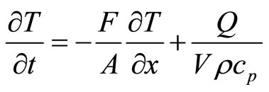 (1)
(1)
Solving a partial differential equation can be hard, so division into discrete units (cascades) is a good approximation with ordinary differential equations. Also it should be noted, that the signal of the differential pressure meter is transformed in a way that it is in linear correlation with the actual flow rate. By merging the constants of the equation, the following form is the result:
 (2)
(2)
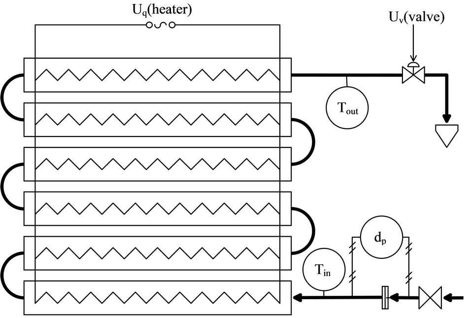
Figure 1. Schematic of the controlled system.
where
 (3)
(3)
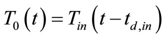
This equation describes the process well, but the MV appears only indirectly in it. To create connection between the valve position and the flow rate the steady-state characteristic was obtained, and it was used as a lookuptable. The relationship of uv and p is zero order with dead time:
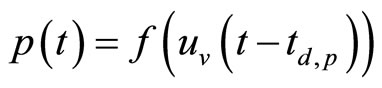 (4)
(4)
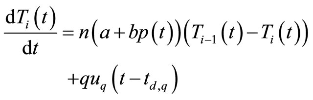
The last step before identification is to discretize the model. Previous studies revealed that the identification may benefit from turning the model to discrete from continuous. The model gets the following form:
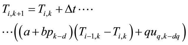 (5)
(5)
Index i marks the number of the cascade, while index k marks the time instance.
The constants a, b, q and dead times td,p, td,q and td, in were subject to identification. A measurement was carries out in which all the inputs changed, but only one at once. The resulting data set was used for identification. Figure 2 shows that the model describes the process very well, and further experiences also justified this model.
3. Constrained Direct Inversion
The studied object is a relative first order system, thus a first order specification is prescribed:
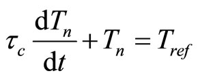 (6)
(6)
τc is the closed-loop time constant. The smaller the τc is, the faster and more aggressive the control becomes. By
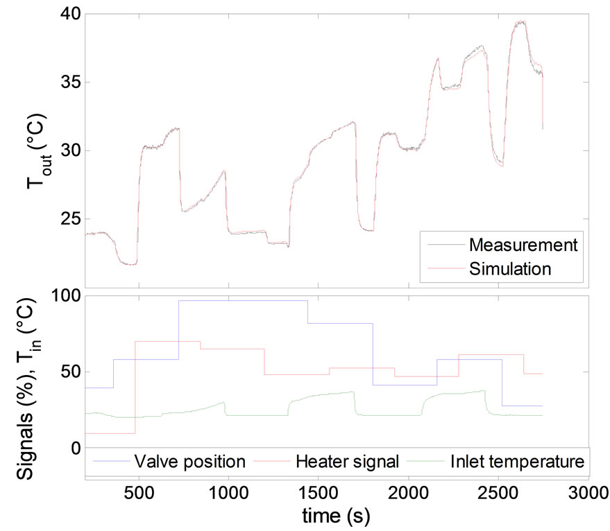
Figure 2. Measurement for identification.
substituting the derivative from the model equation, we get an algebraic equation. It can be rearranged to express the signal p, which is in direct connection with the MV:
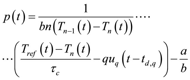 (7)
(7)
The valve position is looked up from the previously obtained steady-state characteristics.
4. Model Predictive Control
This paper is not meant to present a novel MPC method, but rather to use the flexibility of well-known elements. The model behind the MPC is the discrete nonlinear model discussed above. The optimization algorithm is the built in Matlab fmincon function, which was set to use SQP algorithm. The control horizon would be either too small for efficient control or too large for reaching optimality, if the value of the MV would be optimized in every discrete time instance. To overcome this difficulty only some of the points were optimized, while the ones between them were interpolated. The MV after the control horizon was the steady-state value, calculated from the steady-state model. The starting guess of the optimization was the sequence found to be optimal in the previous time instance, with the according time shift. Modeling error is not studied here, thus feedback is not included in the algorithm.
5. The Objective Function and the Closed-Loop Specification
The most widely used objective functions are the sum of squared errors and the sum of absolute errors, although there are numerous other possibilities. Here the squared error is studied, because the main effects are similar with absolute error. As a recent example [8] uses the same objective function for a MIMO case.
Let the cost function be the following:
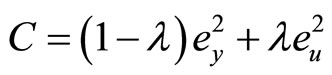 (8)
(8)
where λ is the weighting factor between the control error term  and MV punishment term
 :
:
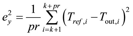 (9)
(9)
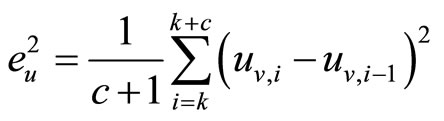 (10)
(10)
pr denotes the prediction horizon, c the control horizon, k the index of the present time sample.
It is important to note, that the errors are averaged in time, thus the differences in control and prediction horizon do not affect the weighting between the two terms. Because of this, the same function can be used for the evaluation of the whole time series. Figure 3 represents a typical simulation experiment, in which both the setpoint and the disturbance changed. Figure 4 shows the numeric values of the cost function obtained with MPC control.
Although MPC optimizes the MV with regards to a short part of the time series, it is still very close the optimality of the whole time series, as the MV found to be optimal has little effect on the CV (and the cost function) outside the prediction horizon.
The question is how these results can be compared to the direct constrained inversion. Constrained inversion of a relative first order system has one degree of freedom, the filtering time constant of the closed-loop specification. By varying the time constant, different cost function values can be obtained for the time series. Further if the λ weighting factor changes, the value of the cost function also changes. The obtained surface is represented on Figure 5. The line marks τc with the lowest cost function at a given λ.
Here we can see the relationship between the closedloop time constant and the λ weighting factor. It is visible, that there is some kind of discontinuity between λ values
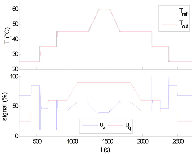
Figure 3. Typical simulation experiment.
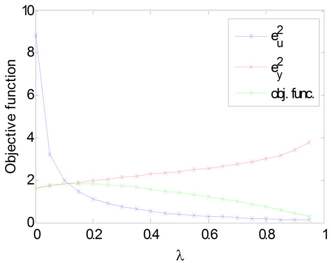
Figure 4. Terms of the objective function with different weighting factors.
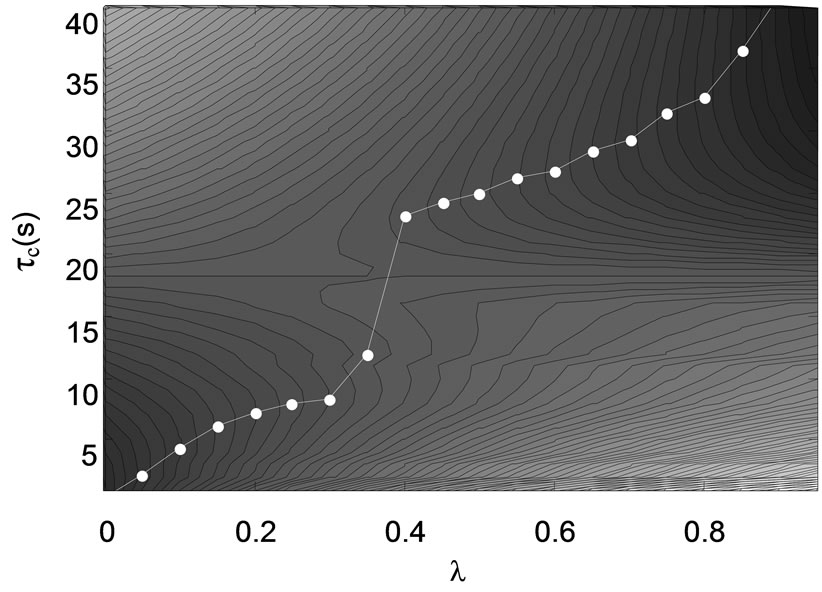
Figure 5. Objective function values achieved by different closed-loop specifications, evaluated with different weighting factors. The lowest value for a given λ is marked with the white line.
of 0.35 and 0.4. The reason is that there are multiple local minimums, and the location of the global minimum is suddenly transferred from one local minimum to another. To understand this effect, let the derivative of the cost function to be equal with zero, which is a necessary condition of optimality:
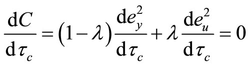 (11)
(11)
By rearranging we get:
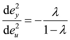 (12)
(12)
Figure 6 represents the relationships of  and
and , and it is visible, that there are inflexion points on this function, meaning that for some λ values the Equation (12) is valid at multiple points. The practical cause for this may be that the optimality can be either approached from the side of fast control or the side of sparing the manipulator. Further local optimums may appear due to manipulator constraints.
On Figure 6 the Pareto-front of the optimization is also visible. The direct inversion method gives a good estimation of the optimality when  can be left high, or otherwise said, the λ is low. However the direct inversion performs badly in decreasing
 , it significantly falls behind the optimality. By applying the available best τc values for a given cost function, the values achievable are presented on Figure 7. These results also assure us that the goodness of the optimality in the case of direct inversion falls below the MPC approach.
The main reason to this effect is that the system, which is nonlinear by its nature, is forced to act as a linear system because of the direct inversion closed-loop specification. This causes sometimes that the system cannot act as fast as desired, and the MV hits the constraints, while in other cases the system would have more reserves to
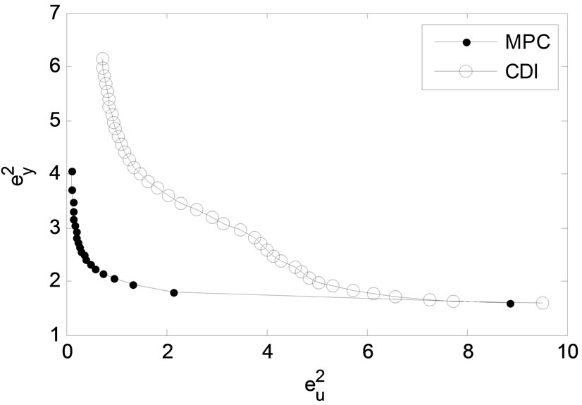
Figure 6. Error of set-point tracking as the function of MV punishment term.
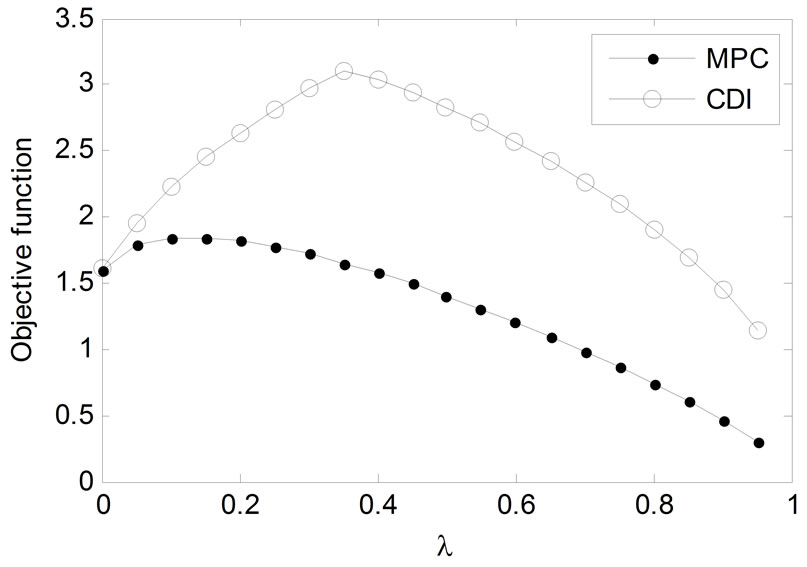
Figure 7. Comparison of achievable optimums while varying the weighting factor.
act faster, but because of the specification this is not exploited. The result is generally more rapid handling of the MV, which results that low  values are hard to be achieved.
The two approaches become similar, when the manipulator constraints rule the controlled system. Figure 8 shows the number of time samples spent on either lower or upper MV constraint. This means that the reserves of the system are totally exploited, and there is no possibility to make the system act even faster. Of course this increases the manipulator punishment term, but when λ is low, this does not increase objective function value significantly.
6. Using Filtered Reference Signal in MPC
Although our primary idea was that the two approaches are very similar in their inversion capabilities, by now a lot of differences were found. To resolve these differences some further changes have to be made on the objective function of the MPC. It is generally accepted to filter the set-point signal to obtain the reference signal in the objective function. The reason for this is the same as including a manipulator punishment term: preserving the stability of the MPC algorithm.
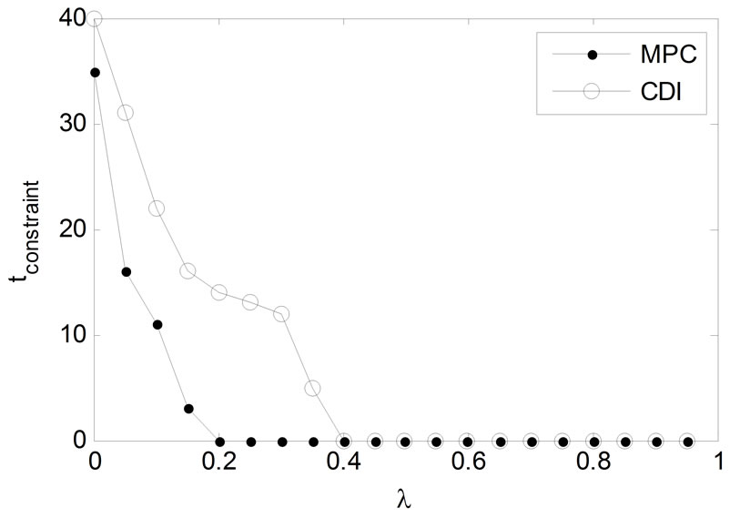
Figure 8. Time spent on constraints as the function of λ.
If λ is set to zero, then only the control error is punished. This way any reference signal can be followed, until MV constraints are not hit. If the same filtering and time shift is applied, as the closed-loop specification of the constrained inversion, then the difference seems to disappear. Still there are some minor sources of difference: numeric inaccuracy of the optimizer, and different handling of constraints. These results are summed up in Figures 9 and 10.
7. Conclusions
Simulation results show that objective function is a key point in optimal control. Even the parameters of the introduced simple objective function can cause significant differences in the behavior of the closed loop. It was also shown, that there are some differences, but with a wellchosen closed-loop time constant, the CDI can act in a very similar way as the MPC does. It is evident that MPC usually performs better in reaching optimality, as the process is evaluated with the same objective function as it was used in its optimization, while CDI follows a rule that is not meant to be an optimal solution. Modifying the reference signal resolves most of the differences. When MV constraints are not hit, MPC and CDI act almost the same.
Finally the source of differences in the two methods can come from different filtering of the reference signal, constraint handling and the difference of numeric and analytic approach. For lower level control it is advantageous to use a fast controller, and as simple as possible. CDI is able to calculate the MV analytically, which is a great advantage when compared to the computationally less efficient or less precise numeric optimization. For more complex systems CDI can also support the optimization of the process by calculating the initial guess that is already close to optimality.
8. Acknowledgements
This work was supported by the European Union and co-
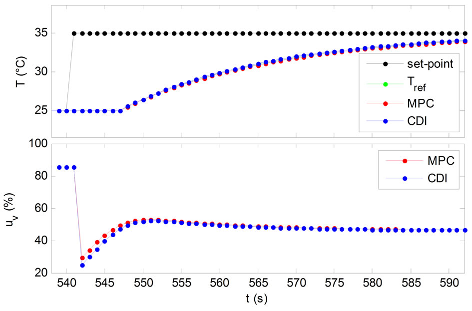
Figure 9. Filtered reference signal applied—both MPC and CDI follow it very tight.
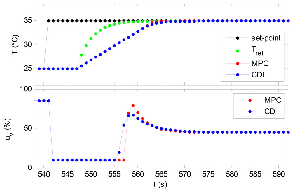
Figure 10. Filtered reference signal, MV constraints active—slight difference between methods.
financed by the European Social Fund in the frame of the TAMOP-4.2.1/B-09/1/KONV-2010-0003 and TAMOP- 4.2.2/B-10/1-2010-0025 projects.
REFERENCES
- G. C. Goodwin, “Inverse Problems with Constraints,” Proceedings of the 15th IFAC World Congress, Barcelona, 21-26 July 2002.
- F. Szeifert, T. Chován and L. Nagy, “Control Structures Based on Constrained Inverses,” Hungarian Journal of Industrial Chemistry, Vol. 35, 2007, pp. 47-55.
- D. Chen and D. E. Seborg, “PI/PID Controller Design Based on Direct Synthesis and Disturbance Rejection,” Industrial & Engineering Chemistry Research, Vol. 41, 2002, pp. 4807-4822. doi:10.1021/ie010756m
- S. Skogestad, “Simple Analytic Rules for Model Reduction and PID Controller Tuning,” Journal of Process Control, Vol. 13, No. 4, 2003, pp. 291-309. doi:10.1016/S0959-1524(02)00062-8
- M. Morari and J. H. Lee, “Model Predictive Control: Past, Present and Future,” Computers and Chemical Engineering, Vol. 23, No. 4-5, 1999, pp. 667-682. doi:10.1016/S0098-1354(98)00301-9
- M. A. Hosen, M. A. Hussain and F. S. Mjalli, “Control of Polystyrene Batch Reactors Using Neural Network Based Model Predictive Control (NNMPC): An Experimental Investigation,” Control Engineering Practice, Vol. 19, No. 5, 2011, pp. 454-467. doi:10.1016/j.conengprac.2011.01.007
- L. R. Tóth, L. Nagy and F. Szeifert, “Nonlinear Inversion-Based Control of a Distributed Parameter Heating System,” Applied Thermal Engineering, Vol. 43, 2012, pp. 174-179. doi:10.1016/j.applthermaleng.2011.11.032
- M. Abbaszadeh, “Nonlinear Multiple Model Predictive Control of Solution Polymerization of Methyl Methacrylate,” Intelligent Control and Automation, Vol. 2 No. 3, 2011, pp. 226-232. doi:10.4236/ica.2011.23027
Nomenclature
NOTES
*Corresponding author.