Intelligent Control and Automation
Vol. 3 No. 2 (2012) , Article ID: 19248 , 10 pages DOI:10.4236/ica.2012.32022
A Geometric Method for Generating Discrete Trace Transition System of a Polyhedral Invariant Hybrid Automaton
1Power and Water Institute, Kermanshah, Iran
2Electrical and Computer Engineering Department, Isfahan University of Technology, Isfahan, Iran
Email: ardalani@ec.iut.ac.ir
Received February 22, 2012; revised March 13, 2012; accepted March 21, 2012
Keywords: Hybrid System; Discrete Trace Transition System; Polyhedral Invariant Hybrid Automata; Discrete Mode Transition Graph
ABSTRACT
Supervisory control and fault diagnosis of hybrid systems need to have complete information about the discrete states transitions of the underling system. From this point of view, the hybrid system should be abstracted to a Discrete Trace Transition System (DTTS) and represented by a discrete mode transition graph. In this paper an effective method is proposed for generating discrete mode transition graph of a hybrid system. This method can be used for a general class of industrial hybrid plants which are defined by Polyhedral Invariant Hybrid Automata (PIHA). In these automata there are no resetting maps, while invariant sets are defined by linear inequalities. Therefore, based on the continuity property of the state trajectories in a PIHA, the problem is reduced to finding possible transitions between all two adjacent discrete modes. In the presented method, the possibility and the direction of such transitions are detected only by computing the angle between the vector field and the normal vector of the switching surfaces. Thus, unlike the most other reachability methods, there is no need to solve differential equations and to do mapping computations. In addition, the proposed method, with some modifications can be applied for extracting Stochastic or Timed Discrete Trace Transition Systems.
1. Introduction
Hybrid dynamical system (HDS) which contains both discrete and continuous dynamics, has attracted considerable attention in recent years [1-3]. Modeling of HDS is a challenging problem because; the model must represent completely both discrete and continuous behavior of HDS and their interactions as well.
A Subclass of hybrid systems that arise naturally in a great number of engineering applications (i.e. DC-DC converters, combustion engines or manufacturing processes), is Discretely Controlled continuous System (DCCS). A typical DCCS consists of a continuous plant (with continuous state vector ) that its operation mode (
 ) is switched by a discrete feedback controller (c.f. Figure 1) [4].
This paper concerns with modeling of a DCCS by a Polyhedral Invariant Hybrid Automaton (PIHA). PIHA is a particular class of Hybrid Automata (HA) that differs from general HA in the following respects:
1) There are no so-called reset mappings associated with the discrete transitions, which means that there are no discontinuities in the continuous state trajectories.
2) The invariant sets are defined by linear inequalities and guards are faces of the invariant sets. A discrete state transition (which is called an internal event) occurs immediately when the continuous state trajectory reaches a guard set [5].
According to the continuity property of the state trajectories in a DCCS, PIHA is a suitable tool for modeling and simulation of DCCS’s [5,6]. An essential step for
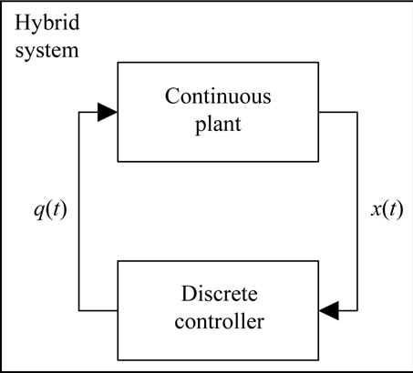
Figure 1. Discretely controlled continuous system.
modeling a DCCS by a PIHA, is obtaining Discrete Trace Transition System (DTTS) of the underling system [7,8]. DTTS is a transition system that abstracts away the continuous dynamics and retains the hybrid system behaviors only at the instants of discrete transitions [5]. Generally speaking, DTTS is a Discrete Event System (DES) that describes all internal events of the DCCS (c.f. Definition 4) and may be represented by a discrete mode transition graph [6].
Obtaining DTTS which is the main contribution of this paper is a challenging problem especially in model based fault diagnosis and supervisory control of DCCS’s. In these applications all internal events must be included in the obtained DTTS to guarantee completeness and efficiency of the model [9]. On the other hand, modeling approach complexity reduces its application in real time and large scale processes [10].
PIHA modeling of DCC has been cited in some lines of researches such as reachability analysis, verification analysis and fault diagnosis of HDS. [4,6,8,11,12]. In these approaches the continuous state space is divided into a set of disjoint partitions so that the union of all partitions covers the entire state space. These methods need complex computations for determining the transitions between elements of the partitions. Computing these transitions needs to solve state equations in each partition which may lead to a high degree of complexity especially for large scale systems [10]. Besides, in some verification analysis, the initial partitions may be refined for several times that it causes more complexity of DTTS computations [5].
Based on the properties of PIHA, especially its continuity property, in this paper a fast geometric method is introduced for detecting DTTS of PIHA with lower complexity. As it will be illustrated in the next section, in a PIHA, invariant sets are linear inequalities; hence guard sets can be visualized as hyper-plans that partition the continuous state space into discrete states. These discrete states, which specify different dynamics of DCCS, are called locations. The locations can be changed under evolution of continuous states. When a continuous state trajectory intersects a hyper-plane guard set, an interval event is occurred and current location is changed. It can be shown that continuity of continuous state trajectories in overall state space restricts the location transitions only to adjacent mode transitions. Therefore, in the DTTS of PIHA only transitions between two adjacent locations are possible. By these considerations, the problem of finding DTTS is reduced to finding all possible adjacent mode transitions [6].
In our proposed method occurrence of these events is detected by computing , where
  is the angle between T and N, which T is the vector field and N is normal vector of switching surface at a guard set point, respectively. For computing T on whole of the switching surface, the surface may be divided into some partitions and T is computed for each one.
The proposed method in this paper has some advantages:
1) There is no need to solve differential equations and T can be computed directly by using state equations.
2) Computations are carried out only on switching surface, instead of the overall state space. It means that the order of the equations reduces at least one order.
3) The method can be easily extended to detect stochastic or timed DTTS.
This paper is organized as follows. Some basic concepts including PIHA and DTTS are defined in section 2. In section 3 our geometric approach for detecting DTTS is described completely. Model completeness and further discussions of the proposed method are presented in section 4. For more illustration, in section 5 the proposed method is applied on a two tank system. And finally in section 6 a brief discussion is given about the abstraction levels.
2. Basic Definitions
In this section the proposed method for detecting DTTS for PIHA is described. Hence, some related definitions are given firstly, and then the method is presented at the end of the section.
Definition 1 [1,5]: A PIHA is a 7-tuple H = (Q, X, f, Init, I, E, G), where
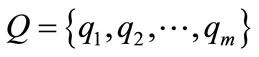 is a set of discrete states or locations;
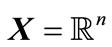 is the continuous state space;
 is a function that assigns to each location
  a vector field
  on X;
on X;
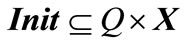 is a set of initial states;
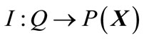 assigns to each location of
  an invariant set of the form
  where
where  is a non-degenerate convex polyhedron;
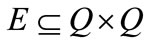 is a set of edges or discrete transitions which are called events;
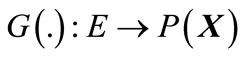 is a guard condition set that assigns to
 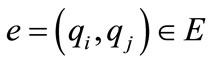 a guard set.
Recall that  (or
(or ) denotes the power set of X.
In PIHA the following assumptions must be satisfied:
1) For each location the guards are the union of the faces of the corresponding invariant set.
2) Events do not lead to transitions that violate invariants.
In addition the following assumption is considered.
• The vector field  is Lipschitz for each location q. This condition implies uniqueness trajectory of
  for each initial state
 .
.
• The hybrid system is a DCCS. This assumption implies that for each location q state equation can be written as  that u denotes input discrete value.
Definition 2 [5]: Given an initial hybrid system state , the continuous trajectory in location q, is
  where
where ; and
; and
 ,
, .
.
(until a discrete transition occurs.)
Definition 3 [1]: A transition system,  , consists of a set of states S;
a transition relation ;
;
a set of initial states .
.
In this paper a PIHA is abstracted into a transition system called Discrete Trace Transition System (DTTS) that abstracts away the continuous dynamics. DTTS is defined as follows.
Definition 4 [6]: For a given PIHA, DTTS is a transition system in which ;
; ;
; ;
;
in which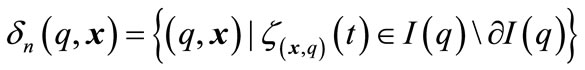 ;
;
 and
and  such that
 ,
,  and
and
 .
.
Here  denotes the boundary of
  and
and  is the interior of
 .
.
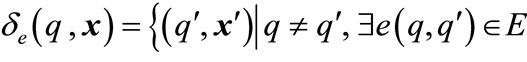
DTTS is a discrete event representation of PIHA and it is used to model transitions of locations and corresponding event sequences. Based on definition 4, DTTS has two parts of transitions , null transition and
 , discrete transition. Null transition comprises all continuous state trajectories that remain in a location indefinitely and discrete transition comprises all continuous state trajectories in the PIHA between different locations.
3. Obtaining DTTS
For detecting DTTS firstly invariants of PIHA must be defined. In this paper invariant sets are determined by using state quantizers. The state quantizer maps the continuous state space  onto discrete states set Q [13]. Here we use rectangular quantizer that leads to hyperboxes as invariant sets. Based on Def. 1 and properties of PIHA, each common face of two hyper-boxes
  and
and  determines a guard set
  that is a subset of a hyper-plane
 . Note that
  for all
  and
and . Figure 2 shows a typical state partition of a two tank system illustrated in section 5. As it is shown in this figure, occurrence of event
  is equal to discrete transition from location
  to location
 .
.
 ,
, . (1)
. (1)
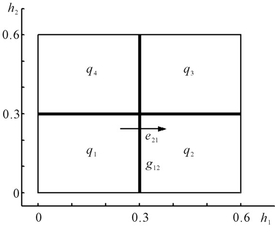
Figure 2. A typical state space partition.
where x, u, d and f denote states, inputs, disturbances and faults respectively.
Based on Def. 1, in PIHA an event  occurs when there is at least an entry point
  for
for  location, in which the continuous trajectory
  intersects with the guard set
 .
.
Generally, finding entry points of all discrete modes, needs to mapping all interior points of each location by solving state equation. These calculations are complex especially when refining partitions is needed [5].
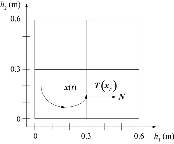
By considering continuity properties of PIHA it is sufficient to check intersection points on guard sets. In fact in our method we assume that each point on a guard set could be an intersection point. This assumption is not a restriction assumption and also guarantees completeness of the obtained model for DTTS that will be considered in the next section. Therefore it is only needed to check that each point on a guard set can be an entry point for location . This test can be carried out by calculating
 , (2)
, (2)
where  is the vector field of
  and
and  is the normal vector of hyper-plane
 , both at
  (c.f. Figure 2). Now it can be deduced that:
 is an entry point for
  if
if  (3)
(3)
Thus the possibility function of occurrence  is defined as
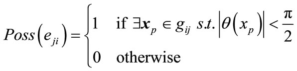 ; (4)
; (4)
Note that in Equation (1)
 . (5)
. (5)
Which can be computed simply by replacing  in
in .
.
By computing Equations (2)-(5) for all , possibility of occurrence
  is determined. Note that if
  for a point
 , then a transition from location
  to location
  is considered in DTTS and there is no need to test other points on
 . By repeating this procedure for all guard sets and for all locations, the overall DTTS of PIHA is detected. This algorithm will be given in the next section, but before that, some major considerations are presented in the next section.
4. Further Discussions
In this section at first completeness of the DTTS is considered and then some special cases that may be arise in obtaining DTTS, are considered.
Completeness of DTTS: Recall that DTTS is a discrete event model for PIHA. Thus DTTS must be a complete model for each initial hybrid state and for each input u. It means that the obtained DTTS could generate all possible discrete trajectories of the underlined DCCS, i.e. . Here,
  and
and  are event trajectories generated by the system and the model, respectively. For investigation the completeness of DTTS, the problem is studied for discrete transition and null transition as follows.
1) Discrete transition: In this case if the point at which event  occurs in HS is
 , then
 . Since during the obtaining procedure of DTTS all points of
  is tested for detecting location transitions, then
  has been considered in DTTS and similarly it is true for all events of HS. Therefore,
  , for all discrete transitions.
2) Null transition: In this case there is no event occurrence at the system and continuous trajectory remains in a location permanently. If  denotes the system event trajectory where tk is the instant time in which a null transition occurs, then we have:
  for all
 . On the other hand By part a), it is resulted that
  for
for . Therefore, for all time
 . (6)
. (6)
Practically, null transition can be detected when all points on guard sets of a location are entry points to this location.
Another issue that is addressed in this section is special cases of the entry point .
.
1) If  for some
 , then
  is an equilibrium point and there is no transition of DTTS in this point (Figure 3(a)).
2) If  for some
 , then
  moves exactly on
  and event
  cannot be detected at this point (Figure 3(b)).
3) If . In this case
  is not continuous at
 . Thus it can be seen that if both
 (a)
(a)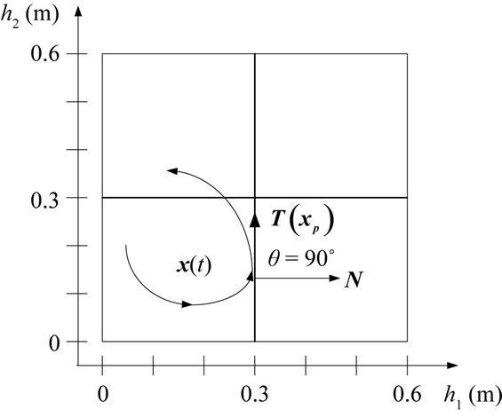 (b)
(b)
Figure 3. Special cases for xp (a) xp is an equilibrium point (T = 0); (b)  and eji cannot be detected at xp.
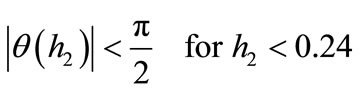
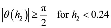
 and
and  are less than
 , then
  is an entry point for pj and the event eji occurs (c.f. Figure 4). But, if
  and
and , then the Zeno phenomenon has occurred at this point. It means that infinite oscillations (i.e. discrete transitions) occur in a finite duration time, thus the point
  is not an entry point.
An important note in this method is that only algebraic equations must be solved and there is no need to solve differential equations. Moreover, since partitions are rectangular, then , for all points on all guard sets In addition; DTTS obtained by this method is complete. At the end of this section the presented method are summarized by following steps:
1) According to state equation and sensor positions, partition the system state space and determine all guard sets.
2) For each guard set choose a set of test points which is called . This set is built by partitioning the guard set and selecting test points from each partition.
3) For a test point, 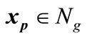 , on the guard set
 ,
,
Figure 4. Discontinuity in  at
at .
.
compute  and
and . If at least one of them is equal to zero, choose another test point from
 , and go to step 3.
4) Compute  and
and  by Equation 2.
If at least one of them is equal to zero, choose another test point, and go to step 3.
5) Determine  or
or  by Equation 4.
6) If  and
and  cannot be detected because of Zeno execution, choose another test point and go to step 3.
7) Repeat steps 3-6 for all test points and for all guard sets.
In this procedure singular points, in which event occurrence cannot be detected, are isolated in steps 3, 4 and 6. If all test points of  are singular points, then another set must be chosen by refining partitions of the guard set. In the next section the proposed approach is simulated to detect DTTS of a two tank system that is a well-known hybrid system.
Limiting Conditions
The main requirement which must be satisfied for applying this method is continuity of state trajectory. Two main situations may contradict this condition:
1) Whenever there is a switching part in the overall system. In this case the presented method could be extended as follows:
a) Represent the switching system by a discrete model such as a Finite State Automaton (FSA).
b) Drive the DTTS of the continuous part c) Obtain the overall DTTS by combining (e.g. synchronized production) of these two discrete models [14].
An example of this situation is considered in the next section.
2) The system is represented by a difference equation set (i.e. it is a discrete system itself). In this case, the discrete model could be derived directly by methods such as cell to cell mapping [9].
5. An Illustrative Example
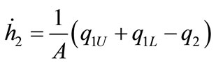
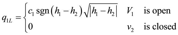
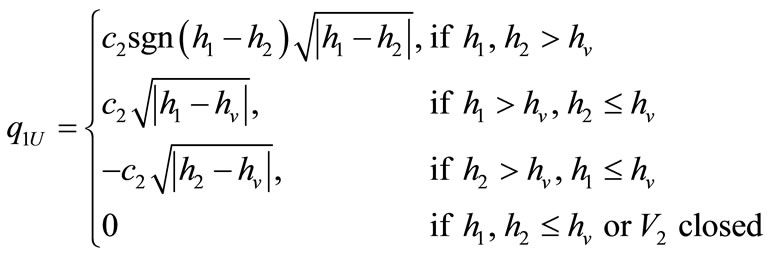
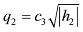
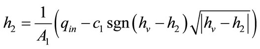
In this section the proposed method is applied for obtaining PIHA of the two-tank system which is affected by faults. The system depicted in Figure 5. This system is a nonlinear hybrid system described by the following differential equations [15,16].
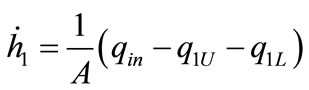 ; (7)
; (7)
 ; (8)
; (8)
 (9)
(9)
 (10)
(10)
 . (11)
Here  and
and  are liquid levels of tank1 and tank2 respectively, qin is input flow and
  is the height of the upper pipe. The other parameters of the system are given in Table 1.
The valves V1 and V2 may be closed or open and the input pump works in on or off mode. The valve V3 is assumed to be always open in the normal operation.
For determining the DTTS of the system, (and consequently its corresponding PIHA), all discrete states and
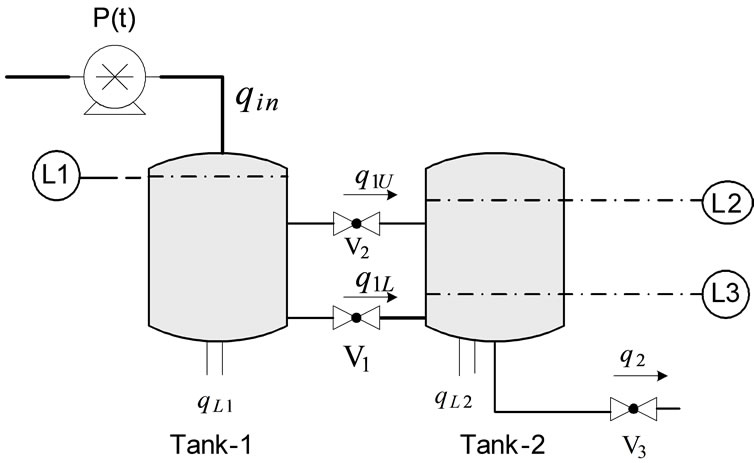
Figure 5. The two tank system.
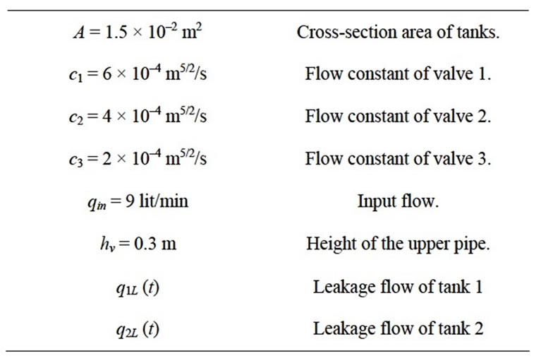
Table 1. Parameters of the two tank system.
events must be identified. DTTS of such systems comprises three parts; Input discrete events, internal events and fault events [6]. Here, Each combination of the situations of the V1, V2 and the pump is considered as a discrete input for the system. Therefore, the system has 8 different discrete inputs which all are assumed to be observable.
In addition, three working modes are considered for the system as follows:
 : Faultless system (faultless).
 : Blockage in the output flow (block2).
 : Leakage in the first tank (leak1).
The crucial part of detecting DTTS is identifying internal events [4]. Here, internal events occur when the liquid levels h1 or h2 reach the height of the upper pipe, hv. At this point, state equations change according to Equations (7)-(10). Thus the state space  is partitioned into four distinct locations due to four distinct dynamics of Equation (10) (c.f. Figure 6).
By considering all discrete states, the PIHA graph of the system is constructed which is shown in Figure 7. In this graph  denotes the sub graph depended on the fault
 ,
,  shows the sub graph related to discrete input
  and
and  denotes the sub graph for fault
  and discrete input
 . It is assumed that the system is in normal mode,
  until the fault
  occurs and the states of the PIHA move towards the
  and remain there. In addition transitions between all
  are assumed to be acceptable.
It can be seen that the basic element of the obtained PIHA, is  which must be determined for all faults and discrete inputs. By considering Figure 6, each
  has 4 invariant sets and the number of all discrete states is equal to:
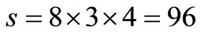 .
.
It is clear that for such a number of discrete states, using the previous methods lead to a huge number of computations. By using the proposed method of this paper these computations reduced to solving a few algebraic
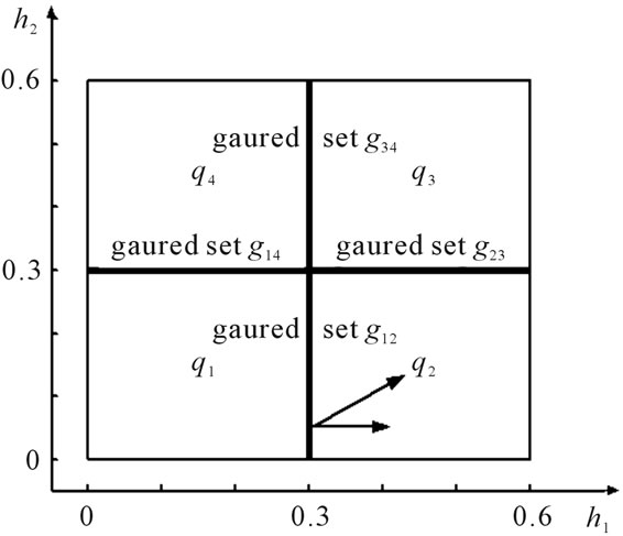
Figure 6. The partitions of two tank system.
equations for a few test points.
For more illustration the detail of the calculations is presented for sub graph Q8,1. In this mode the system is working with no fault, all valves are assumed to be opened and the pump is on. By using our method ,
,  , and,
  is computed for all
  and for all guard sets. For example for guard set
 , and for location 1;
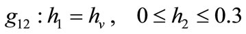 ;
;
 ;
;
Not that the direction of the normal vector for each face of a hyper box is considered into the inside of the hyper box.
 where,
  due to the characteristic of guard set,
  and
and
 .
.
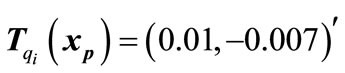
By Equation (2),  is computed for all
  0.3, and is depicted in Figure 8(a). It is seen that:
 ,
,
 .
.
Therefore by using Equation (4), it is resulted that:
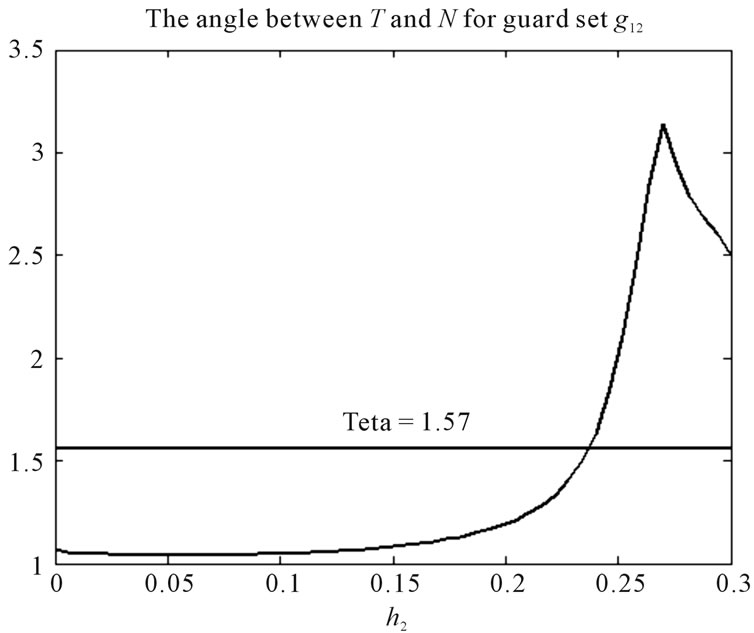
By repeating these computations for the other guard sets,  and possibilities of all events are derived. Figure 8 shows
  for all guard sets and the obtained DTTS is depicted in Figure 9. In this graph nodes denote locations and events are denoted by edges. On each edge the condition for that transition has been written as well.
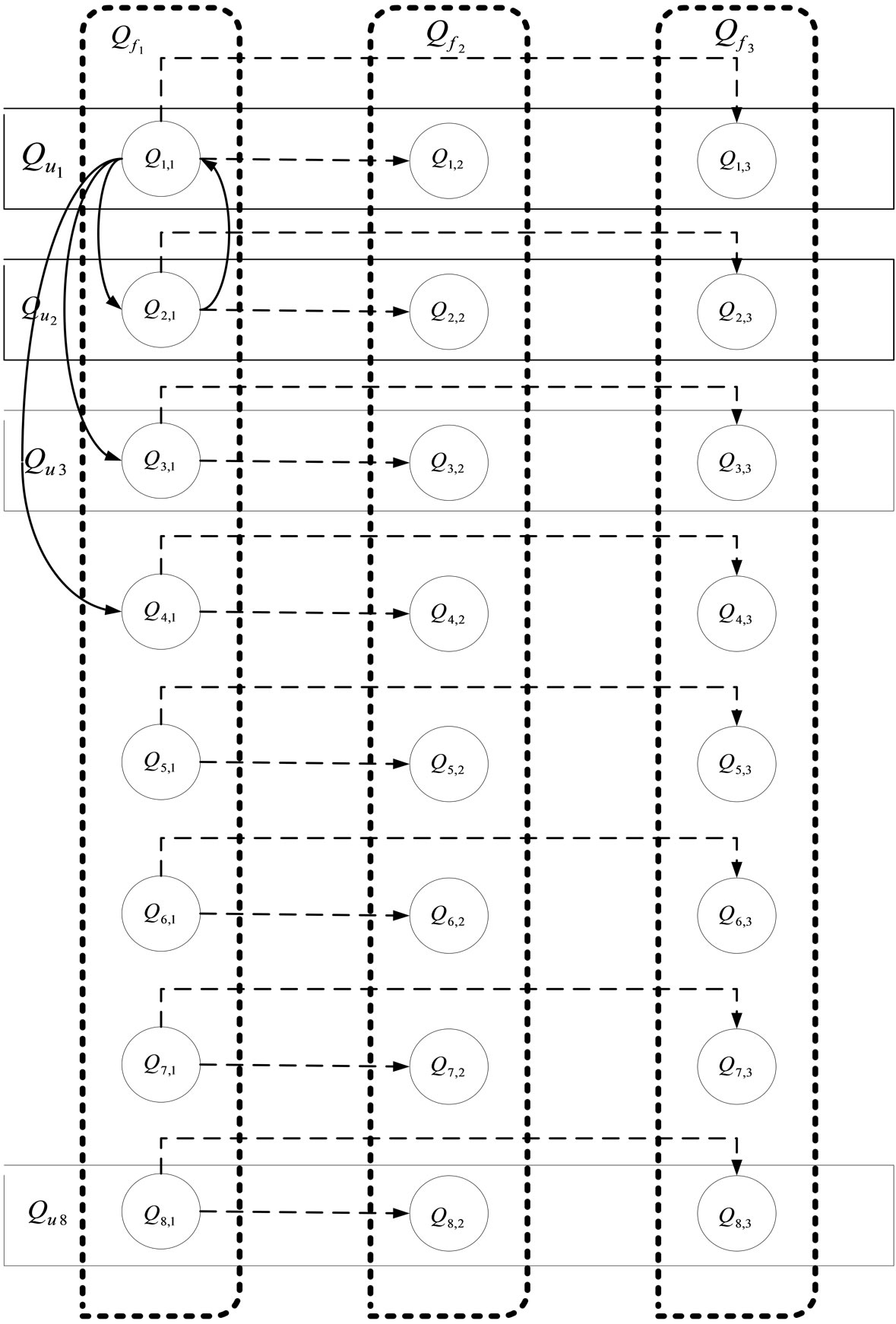
Figure 7. PIHA graph of the two-tank system.
Note that when possibility of an event is 1 for some point on a guard set, there is no need to check other points. Generally, each guard set may be divided into some partitions and these computations are carried for a few points of each partition.
In Figure 9 the edge between nodes 3 and 2, shows that this transition occurs just at . In fact this point can be considered as a guard set and
 is computed for this. Here
 that indicates the transition from location 4 to location 2. For each sub-graph Qi,j, a transition matrix, Li,j would be defined. In this matrix, each entry li,j indicates a state transition from state j to state i. For example the transition matrix for DTTS of Figure 9 is as follows.
 (a)
(a) (b)
(b)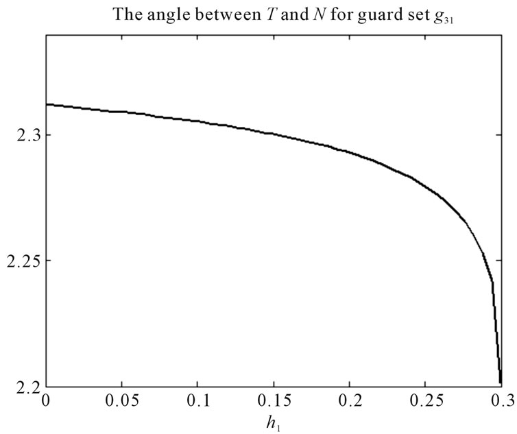 (c)
(c)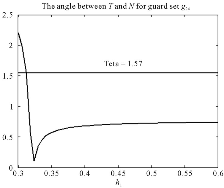 (d)
(d)
Figure 8. θ(x) for guard sets g12, g24, g34 and g31, when all valves are open.
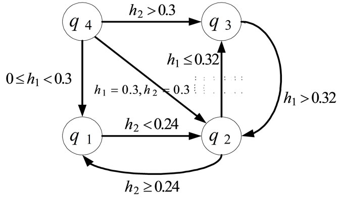
Figure 9. DTTS of two-tank system for Q8,1.
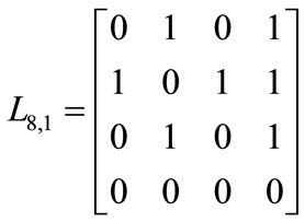 .
.
6. Hierarchical DTTS
The method presented in this paper generates a Finite State Automaton (FSA) as DTTS of a PIHA. In this FSA all continuous behavior of the original system are abstracted by discrete states and their transitions. Such FSA has been used in some fault diagnosis applications, successfully [17,18]. In [16,17] the diagnosability analysis have been presented for such FSA. Generally speaking, a FSA is diagnosable if it could generate eventually, two different discrete trajectories for two different faulty modes. If the obtained FSA (i.e. DTTS) is not diagnosable, it means that the level of abstraction is high and some necessary details have been ignored. In these cases two modifications could be used.
1) Increasing the discrete states by refining the partitions. In this method, some ignored details of the continuous behavior are considered, but the dimension of the FSA is increased [10].
2) Using the other discrete event models for representing the DTTS. In fact, in these approaches, other discrete event models such as Stochastic Automata (SA) or Timed Automata (TA) are applied [13,19]. These models consider more details of the continuous behavior within a location rather than the FSA. In SA the probabilities of the state transitions are considered instead their possibilities. In TA, each discrete state transition is known with its occurrence time. In fact, for abstracting PIHA a hierarchical modeling can be used due to the abstracting level. FSA has the highest degree of abstraction and the most simplicity of calculations. SA is in the second level of the abstraction and TA is in the third level [4].
The presented method in this paper could be extended for SA or TA modeling of DTTS. Basic principles of these extensions are given here briefly, while more details must be considered in each one.
In the case of SA extension, the probability of occurrence of eji is computed by:
 . (12)
Here,  denots the length of the part of g12 in which the event eji occurs and l is the whole length of g12.
The extension of the method for TA modeling could be carried by computing the interval time of reaching a continuous state trajectory to a guard set. Because the computations are done only for some points (or intervals) on the guard sets, then the complexity of calculations is yet lower than the other methods.
7. Conclusions
In this paper a geometric method is presented to detect discrete trace transition system of a PIHA. Since a wide range of technological plants can be described by a PIHA, this method can be used in these areas.
Constructing DTTS of a hybrid system is the first and essential step in analyzing such systems. The method of this paper uses continuity properties of PIHA for detecting DTTS without need to solve differential equations. In addition, the computations are done only on switching surfaces, which have smaller dimensions rather than the original state space. The method can be easily extended to detect stochastic DTTS or timed DTTS.
REFERENCES
- J. Lygeros, “Lecture Notes on Hybrid System,” Department of Electrical and Computer Engineering University of Patras, Patras, 2004.
- W. Wang, D. H. Zhou and Z. Li, “Robust State Estimation and Fault Diagnosis for Uncertain Hybrid Systems,” Nonlinear Analysis: Theory, Methods & Applications, vol. 65, No. 12, 2006, pp. 2193-2215. doi:10.1016/j.na.2006.02.047
- R. Alur, T. A. Henzinger and E. D. Zontag, “Hybrid Systems III. Verification and control (Lecture Notes in Computer Science),” Springer, Berlin, 1996.
- J. Lunze, “Fault diagnosis of Discretely Controlled Continuous Systems by means of Discrete Event-Models,” Discrete Event Dynamic Systems, vol. 18, No. 2, 2008, pp. 181-210. doi:10.1007/s10626-007-0022-3
- A. Chutinan and B. H. Krogh, “Computational techniques for Hybrid System Verification,” IEEE Transactions on Automatic Control, vol. 48. No. 1, 2003, pp. 63- 75. doi:10.1109/TAC.2002.806655
- S. Baniardalani, “Design and analysis of Discrete Event Model Based Fault Diagnosis for a Hybrid System,” Ph.D. thesis, Isfahan University of Technology, Isfahan, 2011.
- R. Alur and T. A. Henzinger, “The Algorithmic Analysis of Hybrid System,” Theoretical Computer Science, vol. 138, No. 1, 1995, pp. 3-34. doi:10.1016/0304-3975(94)00202-T
- J. Lunze and B. Nixdorf, “Discrete reachability of hybrid systems,” International Journal of Control, vol. 76, No. 14, 2003, pp. 1453-1468. doi:10.1080/0020717031000151309
- J. Schröder, “Modeling, State Observation, and Diagnosis of Quantized Systems,” Springer-Verlag, Berlin, 2003.
- D. Forstner and J. Lunze, “Discrete-Event models of quantized system for diagnosis,” International Journal of Control, Vol. 74, No. 7, 2001, pp. 690-700. doi:10.1080/00207170010025276
- S. Ratschan and Z. She, “Safety verification of Hybrid Systems by Constraint Propagation Based Abstraction Refinement,” Hybrid Systems: Computation and Control, Vol. 3414, 2005, pp. 573-589. doi:10.1007/978-3-540-31954-2_37
- G. Frehse, “Algorithmic verification of Hybrid System Past HyTech,” International Journal on Software Tools for Technology Transfer, Vol. 10, No. 3, 2005, pp. 258- 273. doi:10.1007/s10009-007-0062-x
- M. Blanke, M. Kinnaret; J. Lunze and M. Staroswiecki, Diagnosis and fault-Tolerant Control, 2nd edition, Springer, Berlin, 2006.
- C. G. Cassandras and S. Lafortune, “Introduction to discrete Event Systems,” 2nd Eddition, Kluwer Academic Publishers, Dordrecht, 2008.
- J. Askari-Marnani, B. Heiming and J. Lunze, “Control reconfiguration: The cosy Benchmark Problem and Its Solution by means of a Qualitative Model Part of chapter 21 of the final report of the project,” control of complex systems (cosy), 2011.
- J. Lunze, J. Askari, et al., “Three-Tank Reconfiguration Control, Control of Complex Systems,” 2001, pp. 24-283.
- J. Pan and S. Hashtrudi-Zad, “Diagnosability analysis and Sensor Selection in Discrete-Event Systems with Permanent Failures,” Proceedings of the 3rd IEEE Conference on Automation Science and Engineering, Scottsdale, 22-25 September 2007, pp. 869-874.
- M. Sampath, R. Segupta, S. Lafortune, S. K. Sinnamohideen and D. Tenketizis, “Diagnosability of discrete event systems,” IEEE Transactions on Automatic Control, Vol. 40, No. 9, pp. 1555-1575. doi:10.1109/9.412626
- P. Supavatanakul and J. Lunze, “Diagnosis of timed automata: Theory and application to the DAMADICS Actuator Benchmark Problem,” Control Engineering Practice, Vol. 14, No. 6, 2006, pp. 609-619. doi:10.1016/j.conengprac.2005.03.028