Intelligent Control and Automation
Vol. 3 No. 1 (2012) , Article ID: 17578 , 12 pages DOI:10.4236/ica.2012.31010
Sensors and Regional Gradient Observability of Hyperbolic Systems
1Mathematics Department, Faculty of Exact Sciences, University Mentouri, Constantine, Algeria
2MACS Team, Department of Mathematics, Faculty of Sciences, University Moulay Ismail, Meknes, Morocco
Email: {ihebmath, rekkabsoraya, zerrik3}@yahoo.fr
Received August 2, 2011; revised November 3, 2011; accepted November 10, 2011
Keywords: Distributed Systems; Hyperbolic Systems; Observability; Regional Gradient Observability; Sensors; Gradient Reconstruction
ABSTRACT
This paper presents a method to deal with an extension of regional gradient observability developed for parabolic system [1,2] to hyperbolic one. This concerns the reconstruction of the state gradient only on a subregion of the system domain. Then necessary conditions for sensors structure are established in order to obtain regional gradient observability. An approach is developed which allows the reconstruction of the system state gradient on a given subregion. The obtained results are illustrated by numerical examples and simulations.
1. Introduction
For a distributed parameter system evolving on a spatial domain , the notion of regional observability concerns the reconstruction of the initial state on a subregion
  of
of . Characterization results and approaches for the reconstruction of regional state are given in [3,4]. Similar results were developed for the state gradient of parabolic systems in [2]. This led to the so-called regional gradient observability and concerns the possibility to reconstruct the gradient on a subregion
  without the knowledge of the system state. The study of gradient observability is motivated by real applications, the case of insulation problems, also there exist systems for which the state is not observable but the state gradient is observable, example is given in [1].
In this paper we present an extension of the above results on regional gradient observability to hyperbolic systems evolving on a spatial domain . That is to say one may be concerned with the observability of the state gradient only in a critical subregion
  of
of . More precisely let (S) be a linear hyperbolic system with suitable state space and suppose that the initial state
  and its gradient
  are unknown and that measurements are given by means of output functions (depending on the number and structure of the sensors). The problem concerns the reconstruction of the state gradient on the subregion
  of the system domain
 without taking into account the residuel part on
  \
\ .
.
Here, we consider the problem of regional gradient observability of hyperbolic systems and we establish condition that allows the reconstruction of the initial gradient on such a subregion. And the paper is organized as follows.
The second section is devoted to definitions and characterizations of this notion for hyperbolic systems. In the third section we establish a relation between regional gradient observability and sensors structure. The fourth section is focused on regional reconstruction of the initial gradient. In the last section we give a numerical approach, extending the Hilbert Uniqueness Method developed by J.L. Lions [5], and illustrations with efficient simulations.
2. Regional Gradient Observability
Let  be an open bounded subset of
  with a regular boundary
 . Fix
. Fix  and let denote by
  and
and .
.
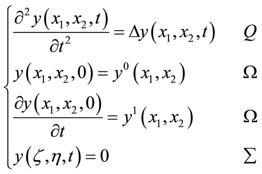
Consider the system described by the hyperbolic equation
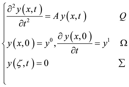 . (1)
. (1)
where  is the second order elliptic linear operator with regular coefficients.
Equation (1) has a unique solution
 [6].
[6].
Suppose that measurements on system (1) are given by an output function:
 . (2)
. (2)
where  is a linear operator depending on the structure of
  sensors.
Let us recall that a sensor is defined by a couple , where
  is the location of the sensor and
  is the spatial distribution of measurements on
 . In the case of a pointwise sensor,
  and
and  is the Dirac mass concentrated in
  see [7].
Let  and
and  then the system
  may be written in the form
 (3)
(3)
with .
.
 has a compact resolvent and generates a strongly continuous semi-group
  on a subspace of the Hilbert state space
  given by

 is a basis in
  of eigenfunctions of
 , orthonormal in
  and
and  the associated eigenvalues with multiplicity
 . Then (3) admits a unique solution
 .
.
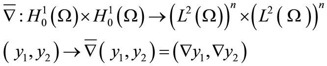
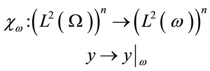
Let us define the observability operator
which is linear and bounded with its adjoint denoted by  and let
  be the operator
where
while their adjoints are denoted by  and
and  respectively.
2.1. Definition 2.1
The system (1) together with the output (2) is said to be exactly (resp. approximately) gradient observable if
Such a system will be said exactly (resp. approximately) G-observable.
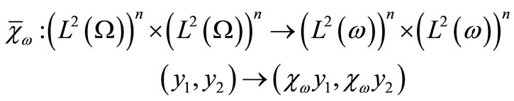
For a positive Lebesgue measure subset  of
of , we also consider the operators
where
and

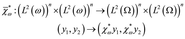
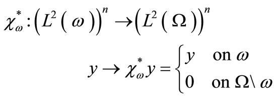
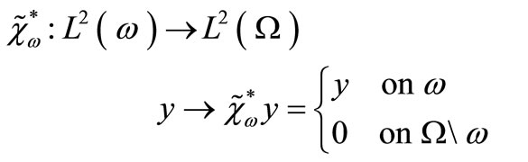
while their adjoints, denoted by ,
,  and
and  respectively and given by
where
and
We finally introduce the operator
 .
.
2.2. Definition 2.2
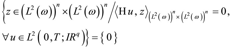
1) The system (1) together with the output Equation (2) is said to be exactly regionally gradient observable or exactly G-observable on  if
if
2) The system (1) together with the output equation (2) is said to be approximately regionally gradient observable or approximately G-observable on  if
if  .
.
The notion of regional G-observability on  may be characterized by the following results.
2.3. Proposition 2.3
1) The system (1) together with the output Equation (2) is exactly G-observable on  if and only if one of the following propositions is holds.
a) For all , there exists
 , such that
b) 
2) The system (1) together with the output Equation (2) is approximately G-observable on  if and only if the operator
  is positive definite.
2.4. Proof
1) a) let us consider the operator  and
and .
.
Since the system is exactly G-observable on , we have
 , and by the general result given in [8], this is equivalent to
  such that
b) Let , then
 ,
,
since the system (1) is exactly G-observable on , there exists
  such that
 .
.
Let put  where
where  and
and  , then
  and
and .
.
Conversely, let , then
  , there exist
and  such that
  and
and  .
.
Since , there exists
such that . Thus
 , which gives
 .
.
2) Let  such that
  .
.
So  which means that
 and since (1) is approximately G-observable then
 , that is
  is positive definite.
Conversely, let  such that
 , then
 , there for
 , that is the system is approximately G-observable on
 .
.
2.5. Remark 2.4
1) If a system is exactly (resp. approximately) G-observable on , it is exactly (resp. approximately) G-observable on
 .
.
2) There exist systems which are not G-observable on the whole domain but may be G-observable on some subregion.
2.6. Example 2.5
Let , we consider the two-dimensional system described by the hyperbolic system
The operator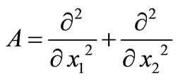 , which the eigenvalues are
 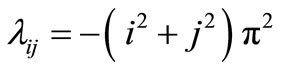 associated to the eigenfunctions
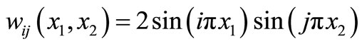 .
.
Measurements are given by the output function
where  is the sensor support and
 is the function measure.
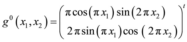
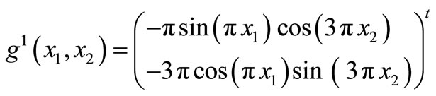
Let the subregion  and we consider the initial state
 ,
,
Then the initial state gradient to be observed is
We have the result.
2.7. Proposition 2.6
The gradient  is not approximately G-observable on the whole domain
 , however it is approximately G-observable on the subregion
 .
.
2.8. Proof
To prove that  is not approximately G-observable on
 , we must show that
 . We have

Since
we have 
and

This gives , and then the system is not approximately G-observable once
 .
.
On the other hand  may be approximately G-observable on
 .
.
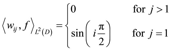
Indeed, suppose that , then
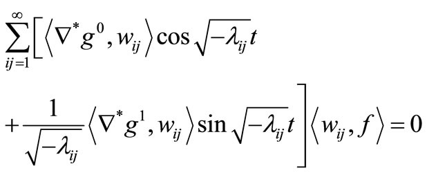
Since for  large enough, the set
 forms a complete orthonormal set of
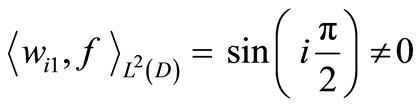
 , we have
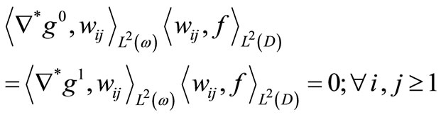
but for  and
and , we have
 .
.
witch gives, 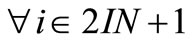
 .
.
But for , we have
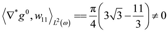 .
.
Thus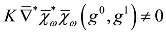 .
.
3. Gradient Strategic Sensors
The purpose of this section is to establish a link between regional gradient observability and the sensors structure.
Let us consider the system (1) observed by  sensors
  which may be pointwise or zone.
3.1. Definition 3.1
A sensor  (or a sequence of sensors) is said to be gradient strategic on
  if the observed system is G-observable on
 , such a sensor will be said G-strategic on
 .
.
We assume that the operator  is of constant coefficients and has a complete set of eigenfunctions in
  denoted by
  orthonormal in
  associated to the eigenvalues
  of multiplicity
 . Assume also that
  is finite, then we have the following result.
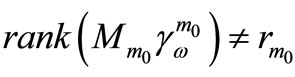
3.2. Proposition 3.2
If the sequence of sensors  is G-strategic on
 , then
  and
and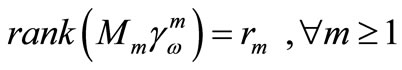 , where
  and
and 
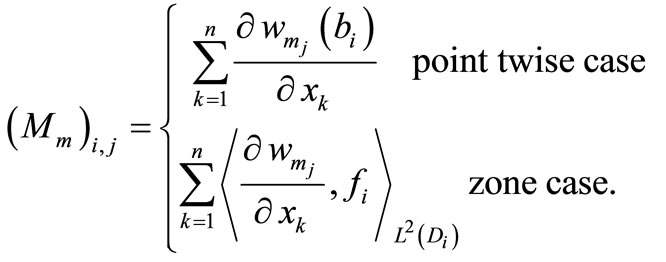 (4)
(4)
and 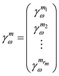
is the row vector the elements of which are with
with  ; for
; for .
.
3.3. Proof
The proof is developed in the case zone sensors.
The sequence of sensors  is G-strategic on
  if and only if
Suppose that the sequence of sensors  is Gstrategic on
  and there exists
 , with
 then there exists
 such that
 and
and . (5)
. (5)
Let  verifying
 (6)
(6)
Let  verifying
 (7)
(7)
and let 
and  then
then
assume that
then
Integrating on  we obtain

and

then

but we have
and
Using the fact that

and
then we obtain 

and
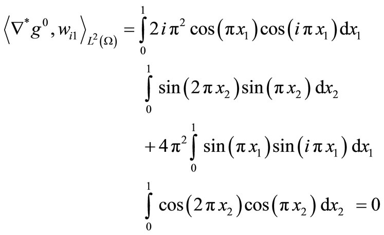
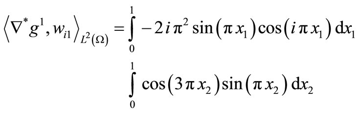
from (5), (6) and (7) we obtain
Thus
this gives ,
,
 and
and , which contradicts the fact that the sequence of sensors is G-strategic.
3.4. Remark 3.3
1) The above proposition implies that the required number of sensors is greater than or equal to the largest multiplicity of eigenvalues.
2) By infinitesimally deforming of the domain, the multiplicity of the eigenvalues can be reduced to one [9,10]. Consequently, the regional G-observability on the subregion  may be possible only by one sensor.
4. Regional Gradient Reconstruction
In this section, we give an approach which allows the reconstruction of the initial state gradient on  of the system (1). This approach extends the Hilbert Uniqueness Method developed for controllability by Lions [6] and don’t take into account what must be the residual initial gradient state on the subregion
 . Consider the set

where 
for , the system
 . (8)
. (8)
has a unique solution
 .
.
We consider the zone sensor case where the system (1) is observed by the output function
 (9)
(9)
 is the sensor support,
  the function of measure and we consider a semi-norm on
  defined by
 (10)
(10)
where  is the solution of (8).
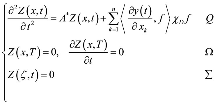
The reverse system given by
 (11)
(11)
has a unique solution
 [5].
[5].
We denote the solution  by
by  and
and
 by
by .
.
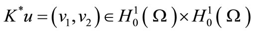
Let consider the operator
where ,
,

and consider the retrograde system which has a unique solution
 (12)
(12)
 [5].
[5].
We denote the solution  by
by  and
and
 by
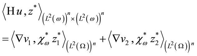
by . Then, the regional gradient observability turns up to solve the equation
 (13)
(13)
where  and
and
 .
.
4.1. Proposition 4.1
If the sensor  is G-strategic on
 , then the equation (13) has a unique solution
  which is the gradient of the initial state to be observed on
 .
.
4.2. Proof
1) Let us show first that if the system (1) is G-observable, then (10) defines a norm on .
.
Consider a basis  of the eigenfunctions of
 , without loss of generality we suppose that the multiplicity of the eigenvalues are simple, then

on  which is equivalent to

The set  forms a complete orthogonal set of
 , then we obtain
and since the sensor  is regionally G-strategic on
 , we have
 then
then .
.
Consequently  and thus
 .
.
Conversely, 
 and
and  (constants), since

and from  on
on , (10) is a norm.
2) Let denote by  completion of
  by the norm (10) and
  be its dual. We show that
  is an isomorphism from
  into
into . Indeed, let
  and
and  the corresponding solution for the problem (8), multiply the first equation of the system (11) by
 , and integrate on
 , we obtain
for the first term, we obtain

Using Green formula for the second term, we obtain

and with the boundary conditions, we obtain

Using Cauchy-Schwartz inequality, we have, 
Hence, 
which proves that  is an isomorphism and consequently the Equation (13) has a unique solution which corresponds to the state gradient to be observed on the subregion
 .
.
4.3. Remark 4.2
The previous approach can be established with similar techniques when the output is defined by means of internal or boundary pointwise sensors.
5. Numerical Approach
In this section we give a numerical approach which leads to explicit formulas for  on
on . We consider the case where the system (1) is observed by the output equation
5.1. Proposition 5.1
If the sensor  is G-strategic on
 , then the initial gradients
  and
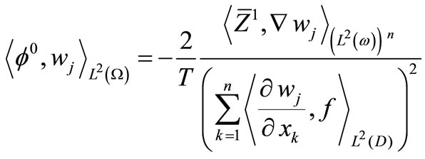
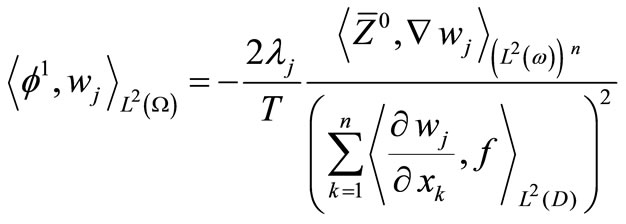
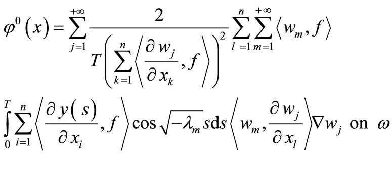
and  may be approached by
  and
and  respectively
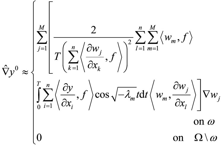 (14)
(14)
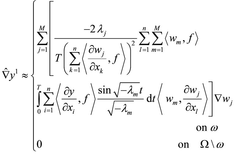 (15)
(15)
where  is an order of truncation.
5.2. Proof
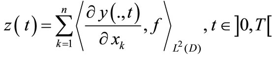
In the previous section, it has been seen that the regional reconstruction of the initial state gradient on  turns up to solve the Equation (13). For that consider the functional
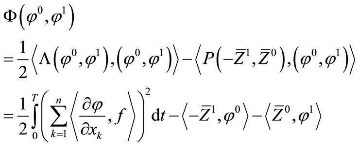
And solving Equation (13) turns up to minimize  with respect to
 .
.
After development and when , we obtain

For  large enough, we have

On the other hand, we have

and
since , then
 on
on  (16)
(16)
and
 on
on  (17)
(17)
we obtain

and

The minimization of (13) is equivalent to solve the two following problems

and

which solutions are, 
 (18)
(18)
and
 (19)
(19)
Now, let  be the solution of the system (12) with

Thus
and
then, we obtain

and

With these developments, according to (18) and (19), we obtain. 
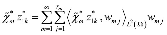
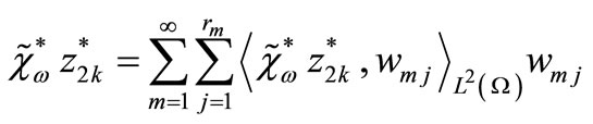
We replace that in the relation (16) and (17), we obtain
and

We consider a truncation up to order , then we obtain the relation (14) and (15).
We define a final error
 .
.
The good choice of  will be such that
 , and we have the following algorithm:
Algorithm
Step 1: Data: The region , the sensor location
  and
and .
.
Step 2: Choose a low truncation order .
.
Step 3: Computation of  and
and  by the formulae (14) and (15).
Step 4: If  then stop, otherwise.
Step 5:  and return to step 3.
5.3. Remark 5.2
If  and
and  are regular enough, we have a regular system state, so measurements may be taken with pointwise sensor. In this case we obtain similar formulaes as in the previous proposition given by
 (20)
(20)
 (21)
(21)
6. Simulations
6.1. Example
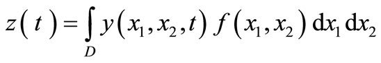
In this section we develop a numerical example that leads to results related to the choice of the subregion, the sensor location and the initial state gradient.
On , we consider the one dimensional system.
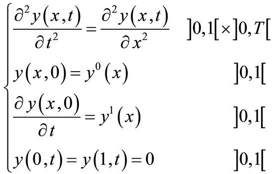 (22)
(22)
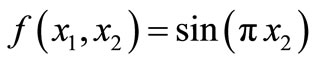
Measurements are given by the output function
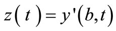 (23)
(23)
The previous system is G-observable on  [7] if and only if
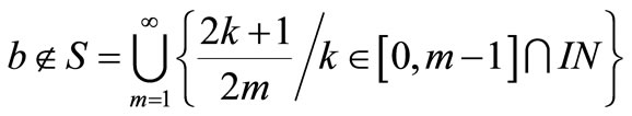
We denote that numerically an irrational number does not exist but it can be considered as irrational if truncation number exceeds the desired precision.
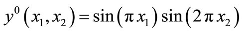
Let , and the sensor is located at
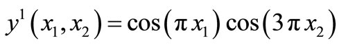
 . The initial gradient to be reconstructed is given by
and
The coefficients  are chosen such that the numerical scheme be stable, and in order to obtain a reasonable amplitude of
  and
and  let us take
  and
and .
.
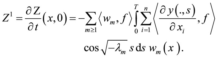
Applying the previous algorithm, using the formulae (20), (21) we respectively obtain the Figures 1 and 2 for  and respectively the Figures 3 and 4 for
 .
.
The estimated gradient is obtained with error  on
on .
.
For , the gradient is reconstructed with error
  on
on .
.
6.2. Simulating Conjectures
Now we show numerically how the error grows with respect to the subregion area. It means that the larger the region is, the greater the error is. The obtained results are presented in Table 1.
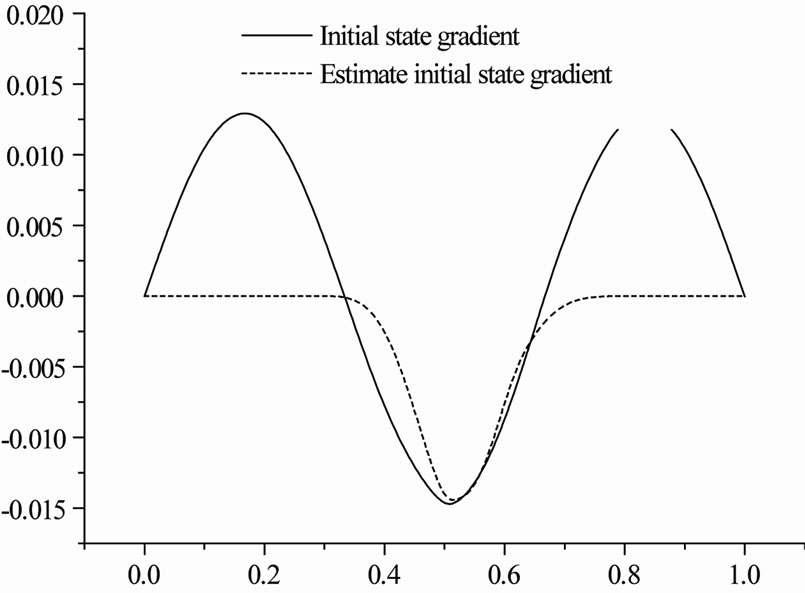
Figure 1. Iheb2.eps: initial state gradient Ñy0 (continuous line) and estimate initial state gradient bar (Ñ)y0 (dashed line).

Figure 2. Nouha2.eps: initial speed gradient Ñy1 (continuous line) and estimate initial speed gradient bar (Ñ)y1 (dashed line).

Figure 3. Iheb1.eps: initial state gradient Ñy0 (continuous line) and estimate initial state gradient bar (Ñ)y0 (dashed line).

Figure 4. Nouha1.eps: initial speed gradient Ñy1 (continuous line) and estimate initial speed gradient bar (Ñ)y1 (dashed line).
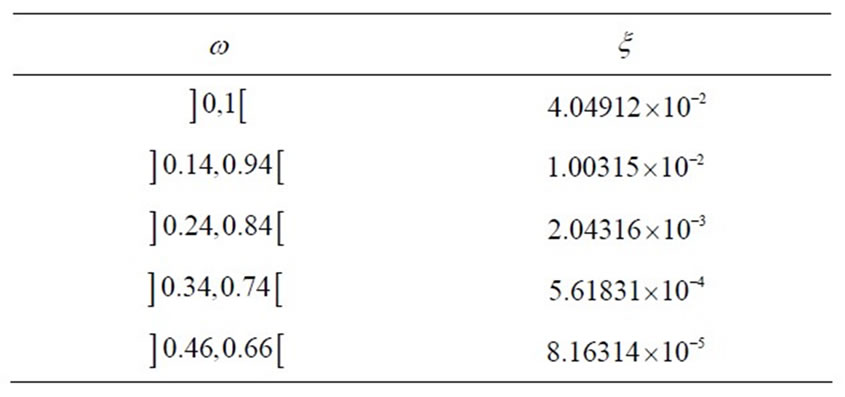
Table 1. Evolution error with respect to the area of the subregion.

Table 2. Evolution error with respect to the initial state gradient amplitude.
Also how both the error decreases with respect to the amplitude  of the initial state gradient. For this let take the subregion
  and
and . We note that the reconstruction error depends on the amplitude of initial state gradient. It means that the greater the amplitude is, the greater the error is. The obtained results are presented in Table 2.
7. Conclusion
Gradient Observability on a subregion interior to the spatial evolution domain of hyperbolic system is considered. A relation between this notion and the sensors structure is established and numerical approach for its reconstruction is given. This allows the computation of the initial state gradient without the knowledge of the system state. Illustrations by numerical simulations show the efficiency of the approach. Interesting questions remain open, the case where the subregion  is part of the boundary of the system domain. This question is under consideration.
REFERENCES
- E. Zerrik, H. Bourray and A. El Jai, “Regional Flux Reconstruction for Parabolic Systems,” International Journal of Systems Science, Vol. 34, No. 12-13, 2003, pp. 641- 650. doi:10.1080/00207720310001601028
- E. Zerrik and H. Bourray, “Regional Gradient Observability for Parabolic Systems,” International Journal of Applied Mathematics and Computer Science, Vol. 13, 2003, pp. 139-150.
- A. El Jai, M. C. Simon and E. Zerrik, “Regional Observability and Sensor Structures,” International Journal on Sensors and Actuators, Vol. 39, No. 2, 1993, pp. 95- 102. doi:10.1016/0924-4247(93)80204-T
- E. Zerrik, “Regional Analysis of Distributed Parameter Systems,” Ph.D, Thesis, University Med V, Rabat, 1993.
- J. L. Lions and E. Magenes, “Problème aux Limites non Homogènes et Applications,” Dunod, Paris, 1968.
- J. L. Lions, “Contrôlabilité Exacte. Perturbation et Stabilisation des Systèmes Distribués,” Dunod, Paris, 1988.
- A. El Jai and A. J. Pritchard, “Sensors and Actuators in the Analysis of Distributed Systems,” In: E. Horwood, Ed., Series in Applied Mathematics, John Wiley, Hoboken, 1988.
- V. Trenoguine, “Analyse Fonctionnelle,” Edition M.I.R., Moscou, 1985.
- A. M. Micheletti, “Perturbazione dello Sopettro di un Elliptic di Tipo Variazionale in Relazione ad uma Variazione del Campo,” (in Italian), Ricerche di Matematica, Vol. XXV Fasc II, 1976.
- A. El Jai and S. El Yacoubi, “On the Number of Actuators in Distributed System,” International Journal of Applied Mathematics and Computer Science, Vol. 3, No. 4, 1993, pp. 673-686.