Circuits and Systems
Vol. 3 No. 3 (2012) , Article ID: 20198 , 9 pages DOI:10.4236/cs.2012.33037
Area and Timing Estimation in Register Files Using Neural Networks
American University of Sharjah, Sharjah, UAE
Email: {asagahyroon, jabdalla}@aus.edu
Received October 30, 2011; revised May 10, 2012; accepted May 17, 2012
Keywords: Register Files; Area Estimates; Timing Estimates; Neural Networks
ABSTRACT
The increase in issue width and instructions window size in modern processors demand an increase in the size of the register files, as well as an increase in the number of ports. Bigger register files implies an increase in power consumed by these units as well as longer access delays. Models that assist in estimating the size of the register file, and its timing early in the design cycle are critical to the time-budget allocated to a processor design and to its performance. In this work, we discuss a Radial Base Function (RBF) Artificial Neural Network (ANN) model for the prediction of time and area for standard cell register files designed using optimized Synopsys Design Ware components and an UMC130 nm library. The ANN model predictions were compared against experimental results (obtained using detailed simulation) and a nonlinear regression-based model, and it is observed that the ANN model is very accurate and outperformed the non-linear model in several statistical parameters. Using the trained ANN model, a parametric study was carried out to study the effect of the number of words in the file (D), the number of bit in one word (W) and the total number of read and write ports (P) on the latency and area of standard cell register files.
1. Introduction
The access time, energy, and area of a register file are critical factors to the performance of modern processors. The access time and size of register files in wide-issue processors often play a critical role in determining cycle time. This is because such files need to be large to support multiple in-flight instructions, and multiported to avoid stalling the wide-issue. Large sized multiport architectures of register files often lead to significant increase in the processor’s power consumption. For example, in the Alpha 21,464, the 512-entry 16-read and 8- write (16-r/8-w) ports register file consumed more power and was larger than the 64 KB primary caches. To reduce the cycle time impact, it was implemented as two 8-r/8-w split register files [1,2].
Register files are heavily-ported RAM structures. A processor capable of issuing eight integer instructions each cycle may need an integer register file with sixteen read ports (corresponding to two source operands per instruction), and eight write ports. It was reported in [3] that the access time for an 80-entry 24-ported register file can exceed 1.5 ns at 0.18 micron technology, potentially being on critical paths determining the cycle time.
Although, the adverse delays effects can be alleviated by pipelining, this complicates the bypass logic instead. In addition, having a deep pipeline increases the branch misprediction penalty, lowering IPC or instructions completed per cycle. Therefore, it is difficult to remove the adverse effect of a large register file completely and it is important to optimize the register file size without performance degradation [4].
The access time of a register file consists of two distinct components: the wire propagation delay and the fan-in/fan-out delay. Register files typically contain long word-lines and bit-lines, which can take a long time to propagate a signal across their length. Bigger register file and an increased number of ports result in a taller register file layout, which translates to longer word-lines and bitlines [5], thereby increasing wire propagation delay. Also, wire delays do not at all scale with the silicon technology improvements. Thus as register files grow in size, with faster transistors (smaller feature sizes), it only exacerbates their delay problem. A circuit diagram for a three ports register file is shown in Figure 1.
Additionally, the physical dimensions of a register file play a very important role in determining its power consumption. They influence the power consumption in more than one way: 1) they determine the length of the wires in the file, hence directly affects the power consumption by determining the capacitance of the nodes, and 2) they impose pipelining constraints, indirectly af-
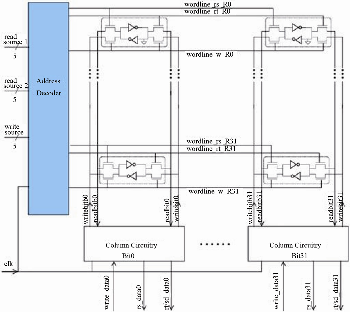
Figure 1. Register file basic circuitry [6].
fecting power by introducing additional power consuming nodes. Therefore, it is critical to have a good model that assists designers in estimating the physical dimensions of these files [7].
Models that can be used to evaluate architectural alternatives in register file design, and assist in making informed decisions prior to the back-end design phase are essential to realizing efficient designs in terms of area, delay, and power.
In recent years, there has been a great advancement in the field of ANN (Artificial Neural Networks), both from theoretical and applications points of view. ANNs have been used in classification, pattern matching, pattern recognition, optimization and control-related problems. In electrical engineering, neural networks have been used to solve a wide variety of VLSI related problems [8-11]. A neural network (NN) approach for modeling the time characteristics of fundamental gates of digital integrated circuits that include inverter, NAND, NOR, and XOR gates is discussed in [8]. The modeling approach presented is technology independent, fast, and accurate, which makes it suitable for circuit simulators. The application of an artificial neural network (ANN) to the study of the nanoscale CMOS circuits is presented in [9]. A novel method of testing analog VLSI circuits, using wavelet transform for analog circuit response analysis and artificial neural networks (ANN) for fault detection is proposed in [10]. Power consumption using neural network of analog components at the system level is discussed in [11]. The proposed method provides estimation of the instantaneous power consumption of analog blocks.
In this work, we propose the use of neural networks to model timing and area for standard cell based register files designed using 130 nm technology. Three parameters that influence the power consumed by a register file, namely, the number of words in the register file (Depth), the number of bits in one word (Width), and the total number of read and write ports (Port) are used as input to the ANN. The output parameters of the ANN are delay and area estimates for the perceived design.
2. Background
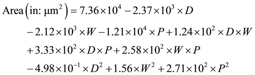
Praveen et al. [12], used low level simulation that takes into account the layout details as well as detailed transistor characterization provided by a standard cell library to collect data on the size and delays exhibited by various structures of register files. They used optimized Synopsys Design Ware components from the UMC130 nm library to design various register files structures. Layouts were generated for register files with a varying number of ports ranging from 3 to 12, a depth that varies from 4 to 64 words, and a width that varies from 8 to 128 bits. All these combinations of register files were designed; patristic capacitances in the routing wires and gate capacitances of each transistor were extracted from the layouts. The extracted netlist was then simulated using ModelSim. After completing over 100 register file design for the 130 nm technology node, the timing and area of each design were tabulated. Curve fitting was performed on each variable using register file depth, width, number of ports, as well as the activity factor as independent input variables. For the designs it is assumed that each of the ports of the register file is driving a load of F04. Equations (1) and (2) below are the derived model equations, where Area and Timing are the subjects of the two equations respectively; the authors in [12] referred to it as the Empire Model. For a complete description of the steps taken to arrive to this model, readers are referred to [12].
 (2)
(2)
In the equations above: D represents the number of words in the file, W represents the number of bit in one word, P represents the total number of ports (read and write). To validate the curve-fitted formulae described by Equations (1) and (2), Praveen et al. in [12], compared them against results from the actual implementations. It is reported that the models exhibit on average about 10% error when compared to the values obtained using detailed simulation.
3. Neural Network Model and Architecture
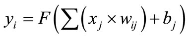
The field of Artificial Neural Networks is one of the main branches of artificial intelligence that found many applications in several engineering disciplines. ANNs are processing elements that are capable of learning relationships between input and output and they can be used for classification, prediction, clustering, and function approximation, among others. Several neural network architectures with different learning algorithms such as backpropagation were used over the years. In general, an ANN consists of massive parallel computational processing elements (neurons) that are connected with weighted connections and have learning capability that simulates the behavior of a brain [13,14]. The network weights and the network threshold values are initially set to random values and new values of the network weights and bias values are computed during the network training phase. The neurons output are calculated using Equation (3) below:
 (3)
(3)
where yi is the output of the neuron i, xj are the input of j neurons of the previous layer; value, wij is the neuron weights, bj is the bias for modeling the threshold; and F is the transfer or activation function [13,14]. The transfer function also known as the processing element is the portion of the neural network where all the computing is performed. The activation function maps the input domain (infinite) to an output domain (finite). The ANN error (E) for a given training pattern i is given by Equation (4):
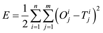 (4)
(4)
where  is the output and
  is the target. For a thorough discussion of neural network theory and applications readers are referred to [13].
The Radial Basis Function (RBF) ANN together with the Gaussian activation function, and the Multi-Layer Perceptron (MLP) together with the hyperbolic tangent (tanh) activation function are among the most widely used feed-forward universal approximators. In this study a hybrid of these two universal approximators is used. Specifically, a RBF ANN topology with one additional hidden layer and 15 neurons (processing elements) in first hidden layer, and four processing element in the second hidden layer are used. The RBF neural network has a Gaussian activation function in the first hidden layer while the additional hidden layer has a linear hyperbolic tangent (linear tanh) activation function and the output layer has a bias axon activation function as shown in Figure 2. The performance of this combination of activation functions for the data set used in this work proved to outperform the standard RBF or standard MLP, when used separately.
As depicted in Figure 2, the neural network architecture used in this study, has one input layer, two hidden layers and one output layer. The input layer consists of three nodes, mainly, the number of words in the register
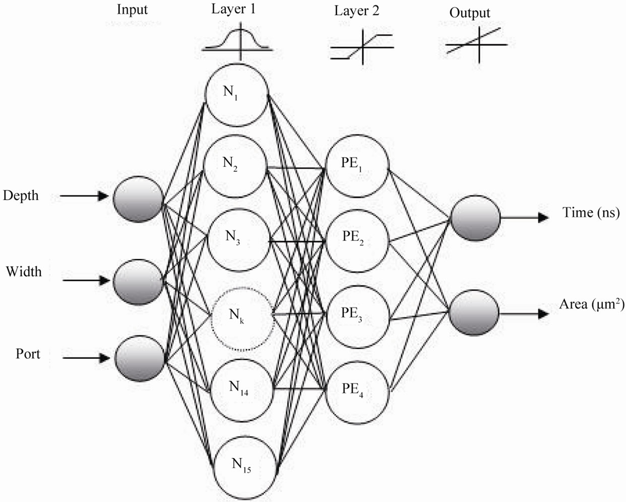
Figure 2. A multilayer RBF neural network topology.
file depth (D), the number of bits in one word width (W), and the total number of read and write ports (P). The output layer of the ANN consists of two nodes which are the time and the area estimates.
To train the NN, data collected from details simulation runs in [12] is divided into two categories, namely, the training data set and, the testing data set. For both sets the maximum Depth value used is 64 registers per file, the minimum is 4; the maximum width used is 64 bits and the minimum is 8, while for the ports parameter the maximum number of ports is 12 ports, and the minimum is 3 ports. For the training data set, the maximum timing computed is 7.55 nano-second (ns) and the minimum is 1.11 ns, while for the test data set, the maximum timing within the used set is 4.92 ns, and the minimum is 1.81 ns. The areas range is 721,383 μm2 to 2512 μm2 for the training set, and 164,590 μm2 to 4902 μm2 for the test set.
Initial random values are used for the weights of the neural network and different learning rates (step sizes) were used for the different layers of the RBF neural network. The learning rate used for the first and second hidden layers is 1.0 and for the output layer is 0.1. A momentum factor of 0.7 was used for the model all through with a back-propagation learning algorithm. The total number of data items used for training the neural network is 60 and the number of data items used for testing the neural network is 20. The neural network was trained four times with 2000 epochs in each training cycle and the average performance was taken. The computed average Normalized Mean Square Error (NMSE) for the training data was 0.00494 with a standard deviation of 0.000614. Figure 3 shows the convergence rate of the four training runs. There is a sharp decrease in the NMSE during the first 15 epochs. As the number of epoch increases, the MSE remains almost constant.
4. Results and Discussions
The ANN model was trained using 60 data sets and for verification the trained ANN model is tested next using 20 randomly selected testing data sets. Parameters of the 20 test data sets were also used to predict the time and area using the Empire model. Tables 1 and 2 show the performance indicators of the 20 testing samples. As shown
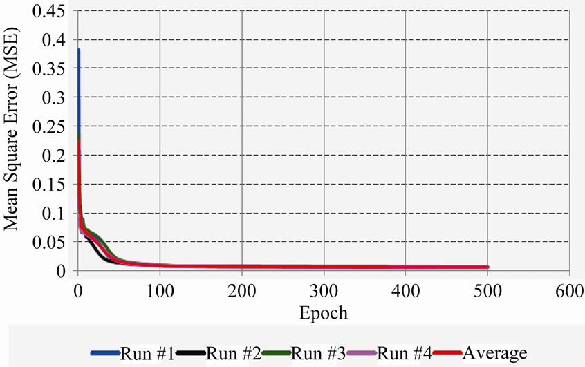
Figure 3. Training NMSE for the four runs of ANN models.
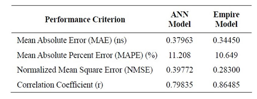
Table 1. Performance of the ANN on time prediction of the test data.

Table 2. Performance of the ANN on area prediction of the test data.
in Tables 1 and 2, the Normalized Mean Square Error (NMSE) is 0.3977 and 0.0261 and the correlation co-efficient (r) is 0.7983 and 0.9872 for time and area, respectively. This indicates that the measured and the ANN predicted values correlate very well for the area and to a lesser extent for the time. The performance of the Empire model is slightly better than the performance of the ANN in all performance criteria in predicting time, however, the ANN model outperformed the Empire model by far in all performance criteria in predicting area estimates.
Table 3 shows the prediction and accuracy of the ANN model and the Empire model based on the test data set as compared to the measured values of time. In column 1, the case number specifies the depth (D), width (W), and number of ports (P) for each design tested. It is observed that 55% of the ANN model predictions of the test data are within 10% or less of the measured values of time compared to 50% of Empire model predictions of the test data are within 10% of the measured values of time. Furthermore, 80% of the ANN predictions of the test data are within 20% of the measured values of the time while 90% of Empire model predictions of the test data are within 20% of the measured values of time. It is clear that the Empire predictions of time are slightly better than the ANN model prediction which corroborate with the results from the performance criteria presented earlier.
Table 4 shows the prediction and accuracy of the ANN model and the Empire model based on the test data set as compared to the measured values of area. It is observed that 45% of ANN model predictions are within
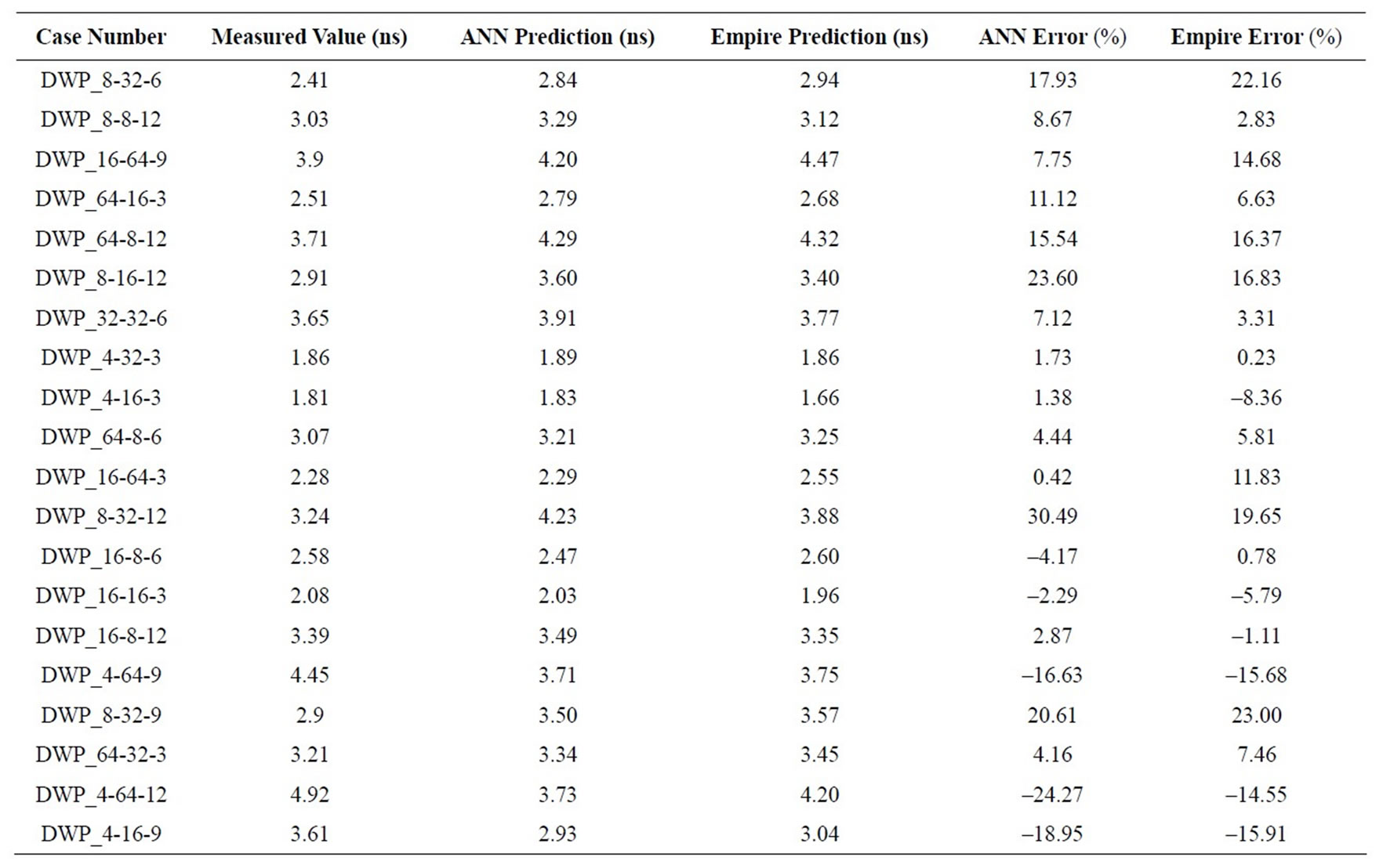
Table 3. Prediction and accuracy of time of test data.
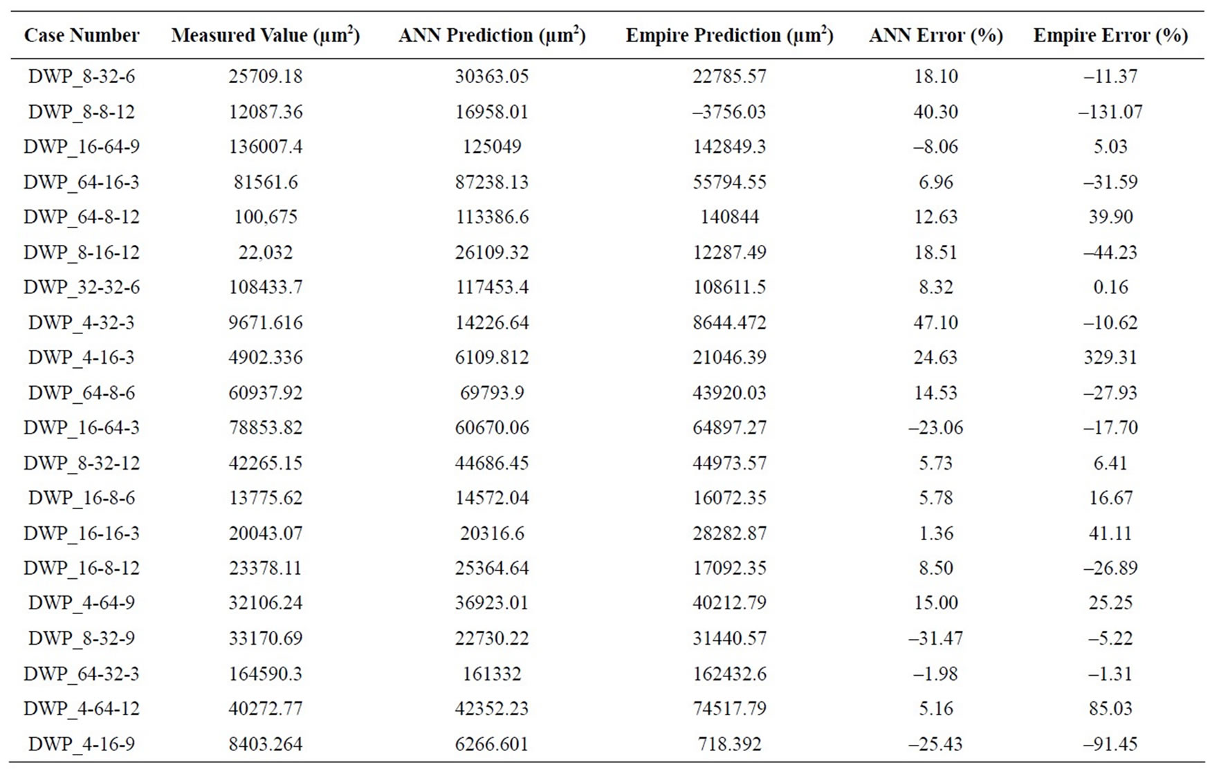
Table 4. Prediction and accuracy of area of test data.
10% or less of the measured values of area compared to 25% of Empire model predictions of the test data are within 10% of the measured values of area. Also, 70% of the ANN predictions of the test data are within 20% of the measured values of the area while only 45% of Empire model predictions of the test data are within 20% of the measured values of area. It is clear that the ANN predictions of area are better than the Empire model predictions. This corroborates the results of the performance criteria presented earlier in Table 1.
Parametric Study
To further compare the performance of the Empire model and the ANN model in predicting the time and the area, we varied the input parameters (width, ports, and depth) and computed the resulting outputs for 6 designs. Figures 4 and 5 depict comparative plots showing the predictions of time and area respectively for varied combinations of parameters.
From Figures 4(c) and (d), it is clear ANN model predictions are fairly accurate when the number of ports is varied with a fixed depth and width. Figure 3(b) shows that the ANN model when the width is increased with the depth and ports parameters fixed has underestimated the time specially with wider designs. Similarly, when the depth is varied while keeping the width and ports fixed (Figures 4(e) and (f)), the ANN predications were relatively above and below the experimental values in few cases.
In the instances selected for area comparison (Figure 6), both models performed relatively well and the predicted areas were close to the experimental values obtained from detailed simulation. However, overall and as the statistical results of Table 2 indicate, the ANN model has outperformed the Empire in area prediction.
From the aforementioned analysis of results and validation of the ANN model, it is evident that the proposed ANN model can be used to provide designers with representative estimates of the time and area of a perceived register file design before committing to silicon. The time and the area estimates for all the register file designs used in this study with 130 nm technology and a supply voltage of 1.2 V are shown in Figures 6 and 7 respectively.
5. Conclusions
The continued trend in microprocessors design towards wider instruction issue and large instruction windows implies register files will have to be designed with large sizes and a large number of read/write ports. Consequently, this will lead to additional power consumption by these large-sized files and a noticeable impact on cy-
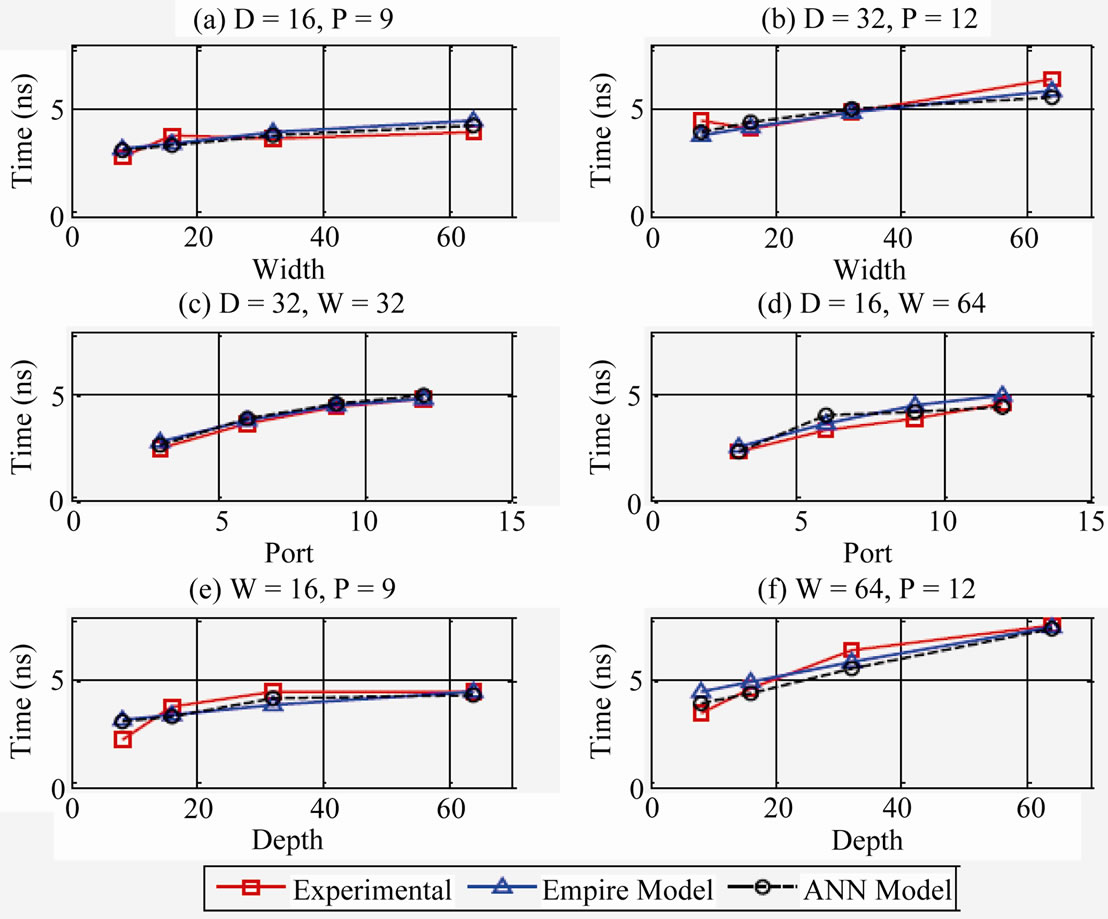
Figure 4. Comparison of time for selected register files.
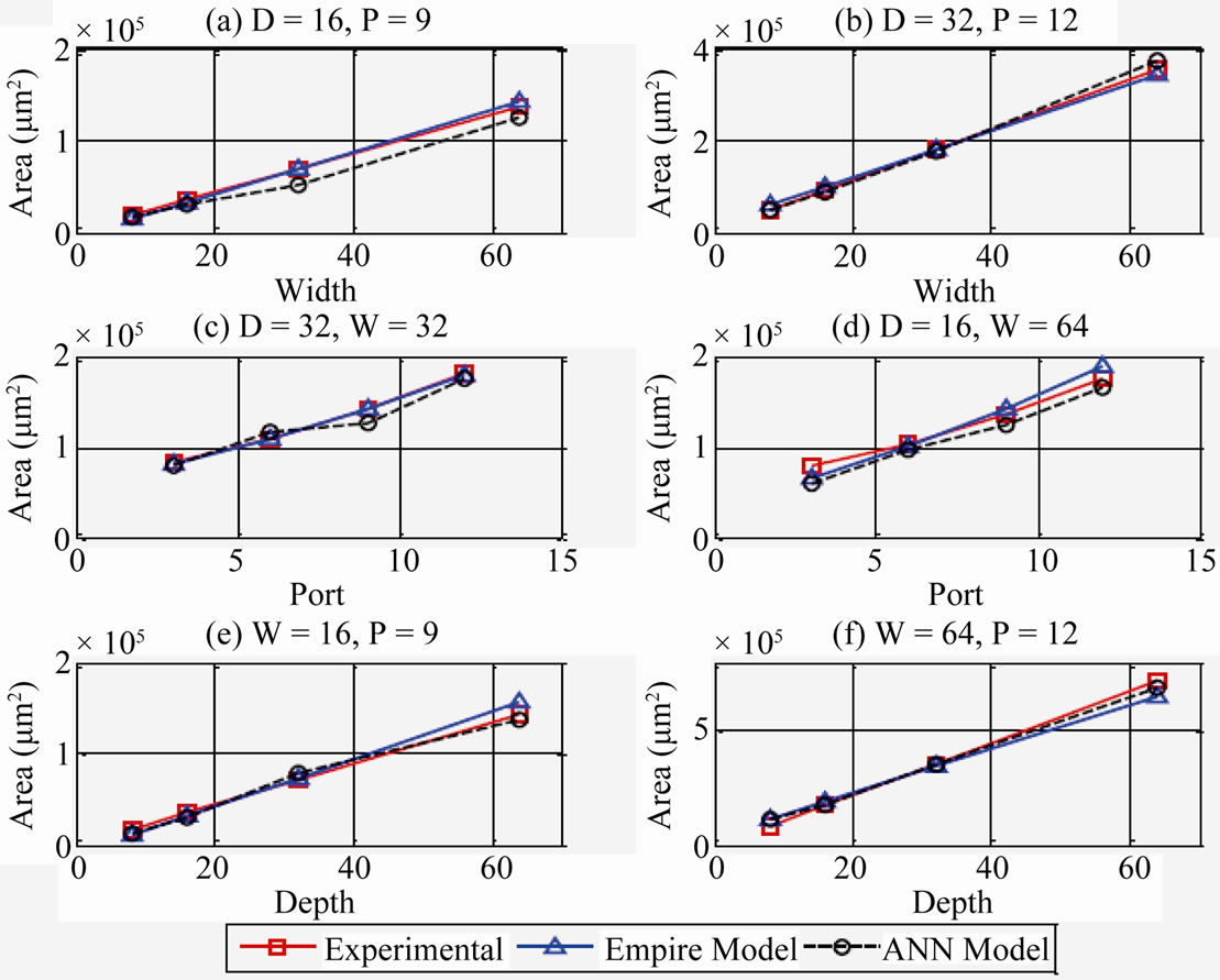
Figure 5. Comparison of area for selected register files.
cle time. Therefore, models and tools that allow designers to predict the area and the timing of a given design prior to committing to silicon are of great benefit to microprocessors designers. Evaluating architectural tradeoffs early in the design cycle provides designers with insight into the performance of a design, and shortens the time-to-market window.
In this paper, we proposed a novel neural network model for estimating the timing and size or area for register file designs. The model is simple and efficient and can be used to provide estimates that are close to those expected when detailed and time consuming simulation is performed. The model is validated by comparing its results to those produced by low level simulation, as well as by comparing it to the recently reported Empire model [11].
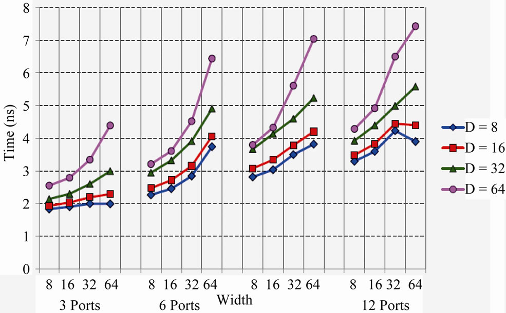
Figure 6. ANN model for time for all ports.
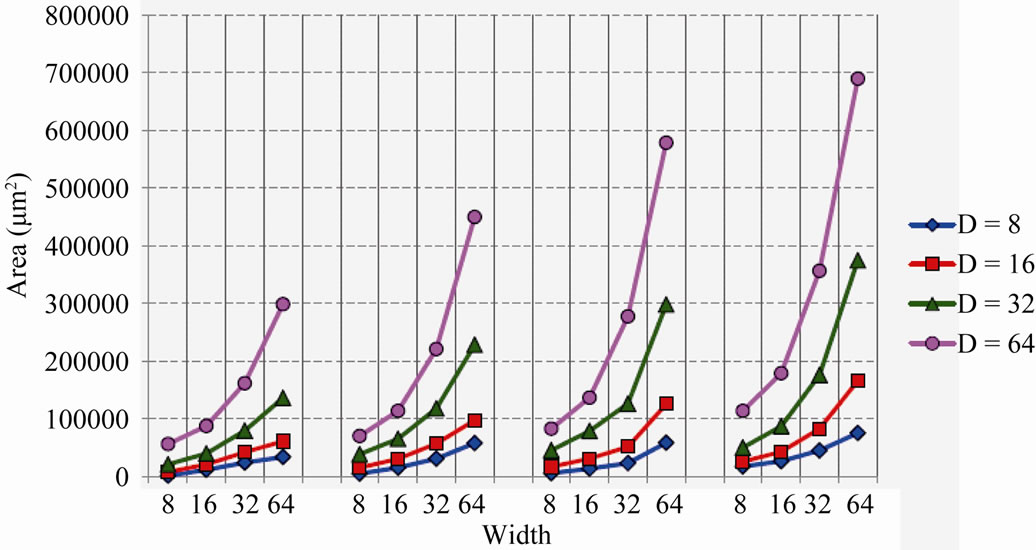
Figure 7. ANN model for area for all ports.
6. Acknowledgements
The authors would like to thank Dr. Praveen Raghavan of IMEC in Belgium for providing the register file designs data for the 130 nm technology node.
REFERENCES
- R. Preston, et al., “Design of an 8-Wide Superscalar RISC Microprocessor with Simultaneous Multithreading,” SolidState Circuits Conference, Vol. 1, 7 February 2002, pp. 334-472.
- N. S. Kim and T. Mudge, “The Microarchitecture of a Low Power Register File,” Proceedings of the 2003 International Symposium on Low Power Electronics and Design, Seoul, 25-27 August 2003, pp. 384-389.
- R. Balasubramonian, S. Dwarkadas and D. H. Albonesi, “Reducing the Complexity of the Register File in Dynamic Superscalar Processors,” Proceedings of the 34th annual ACM/IEEE International Symposium on Microarchitecture, Austin, 1-5 December 2001, pp. 237-248.
- Y. Tanaka and H. Ando, “Reducing Register File Size through Instruction Pre-Execution Enhanced by Value Prediction,” Proceedings of the 2009 IEEE International Conference on Computer Design, Nagoya, 4-7 October 2009, pp. 238-245. doi:10.1109/ICCD.2009.5413149
- S. Rixner, W. J. Dally, B. Khailany, P. Mattson, U. J. Kapasi and J. D. Owens, “Register Organization for Media Processing,” Proceedings of the 6th International Symposium on High Performance Computer Architecture, Stanford, January 2000, pp. 375-386.
- J. Tseng and K. Asanovic, “Energy Efficient Register Access,” Proceedings of the 13th Symposium on Integrated Circuits and Systems Design, Cambridge, 2000, pp. 377-382.
- K. M. B Ahin, P. Patra and F. N. Najm, “ESTIMA: An Architectural-Level Power Estimator for Multi-Ported Pipelined Register Files,” Proceedings of 2003 International Symposium on Low Power Electronics and Design, Hillsboro, 25-27 August 2003, pp. 294-297.
- N. Kahraman and T. Yildirim, “Technology Independent Circuit Sizing for Standard Cell Based Design Using Neural Networks,” Digital Signal Processing, Vol. 19, No. 4, 2009, pp. 708-714. doi:10.1016/j.dsp.2008.11.009
- F. Djeffal, M. Chahdi, A. Benhaya and M. L. Hafiane, “An Approach Based on Neural Computation to Simulate the Nanoscale CMOS Circuits: Application to the Simulation of CMOS Inverter,” Solid-State Electronics, Vol. 51, No. 1, 2007, pp. 48-56. doi:10.1016/j.sse.2006.12.004
- P. Kalpana and K. Gunavathi, “Wavelet Based Fault Detection in Analog VLSI Circuits Using Neural Networks,” Applied Soft Computing, Vol. 8, No. 4, 2008, pp. 1592- 1598. doi:10.1016/j.asoc.2007.10.023
- A. Suissa, O. Romain, J. Denoulet, K. Hachicha and P. Garda, “Empirical Method Based on Neural Networks for Analog Power Modeling,” IEEE Transactions on Computer-Aided Design of Integrated Circuits and Systems, Vol. 29, No. 5, 2010, pp. 839-844. doi:10.1109/TCAD.2010.2043759
- P. Raghavan, A. Lambrechts and M. Jayapala, F. Catthoor and D. Verkest, “EMPIRE: Empirical Power/Area/ Timing Models for Register Files,” Microprocessors and Microsystems, Vol. 33, 2009, pp. 295-300. doi:10.1016/j.micpro.2009.02.009
- S. Haykin, “Neural Networks: A Comprehensive Foundation,” 2nd Edition, Prentice-Hall, Upper Saddle River, 1999.
- J. A. Abdalla and R. A. Hawileh, “Modeling and Simulation of Low-Cycle Fatigue Life of Steel Reinforcing Bars Using Artificial Neural Network,” Journal of the Franklin Institute, Vol. 348, No. 7, 2011, pp. 1393-1403. doi:10.1016/j.jfranklin.2010.04.005