Circuits and Systems
Vol.3 No.1(2012), Article ID:16611,10 pages DOI:10.4236/cs.2012.31010
Floquet Eigenvectors Theory of Pulsed Bias Phase and Quadrature Harmonic Oscillators
Department of Information Engineering, Electronics and Telecommunications, Sapienza Università di Roma, Rome, Italy
Email: {palma, perticaroli}@die.uniroma1.it
Received September 19, 2011; revised October 26, 2011; accepted November 5, 2011
Keywords: Floquet Eigenvectors Noise Decomposition; Phase and Quadrature Oscillators; Pulsed Bias Oscillator; Oscillator Phase Noise
ABSTRACT
The paper presents an analytical derivation of Floquet eigenvalues and eigenvectors for a class of harmonic phase and quadrature oscillators. The derivation refers in particular to systems modeled by two parallel RLC resonators with pulsed energy restoring. Pulsed energy restoring is obtained through parallel current generators with an impulsive characteristic triggered by the resonators voltages. In performing calculation the initial hypothesis of the existence of stable oscillation is only made, then it is verified when both oscillation amplitude and eigenvalues/eigenvectors are deduced from symmetry conditions on oscillator space state. A detailed determination of the first eigenvector is obtained. Remaining eigenvectors are hence calculated with realistic approximations. Since Floquet eigenvectors are acknowledged to give the correct decomposition of noise perturbations superimposed to the oscillator space state along its limit cycle, an analytical and compact model of their behavior highlights the unique phase noise properties of this class of oscillators.
1. Introduction
Quadrature oscillators may represent important components of integrated digital modulations transceivers. The huge demand for wireless communications has indeed led to develop compact and low power circuits in order to reduce both implementation costs and devices consumptions. The need of precise quadrature signals can be found for example in low-IF or direct conversion modemodulator architectures. A quadrature oscillator can easily fit such request avoiding the use of a dedicated circuitry in conjunction with a single standard oscillator. However there are still many issues with quadrature oscillators concerning in particular the relation between phase noise and quadrature error [1]. In authors opinion, quadrature oscillators should be regarded a coupled system in the whole and this aspect increment the difficult of a theoretical noise treatment.
In this paper we propose to achieve a full analysis of a new phase-quadrature architecture based on pulsed bias we recently presented in [2]. This aim matches with the general effort toward the reduction of phase noise in oscillators. Stimulated from the idea of Hajimiri-Lee [3] and even dating back from the Colpitts oscillator, pulsed bias in oscillators represents a new attractive solution attempting to concentrate the necessary energy refill in the portion of the oscillator limit cycle where noise projection on the first Floquet eigenvector (thus the contribution to the phase noise close to the fundamental) is minimum.
The main properties of this class of harmonic oscillators architecture are derived through an analytical treatment based on Floquet eigenvectors noise decomposition. Floquet eigenvectors approach is indeed acknowledged as a correct analytical methodology for the description of noise perturbations [4].
In addition Coram [5] remarked that the correct noise decomposition is obtained following eigenvectors relative orientation. Floquet eigenvectors determination is then necessary in order to produce a consistent noise analysis. We notice that, since in a pulsed bias architecture the pulse itself modifies eigenvectors, even the choice of an eventual optimal position of the bias pulse is not simply determinable [6]. Hence the calculation we present must take into account the mutual dependence of bias pulse and eigenvectors. Following this approach we derive an analytical formulation which allows to point out some important properties of this class of oscillators:
1) the orthogonal dynamic of coupled oscillators;
2) the minimization of noise introduced by the bias pulse due to minimum projection on first eigenvector;
3) the intrinsic orthogonality of eigenvectors which ensures minimization of noise contribution from parasitic resistances in resonators.
2. Oscillator Model
The simplified model we refer to is reported in Figure 1. It presents only four state variables corresponding to capacitors voltages and inductors currents of two identical RLC resonators and referred respectively as OSC_I and OSC_Q. The resulting state vector is 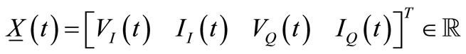 . Here and in the following all vectors and parameters quantities are in real numbers field if not differently specified. Coupling between resonators in a positive feedback configuration is accomplished by pulsed current generators emulating active devices. This model can be seen as a rather drastic simplification of a real oscillator, however if we assume the parasitic introduced by transconductors to be much smaller than those in resonators they can be merged in resonators themselves, thus avoiding to increment the effective space state dimension.
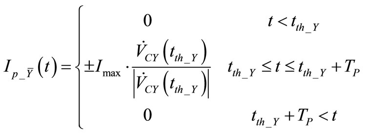
The model assumes a current pulse of fixed duration injected in the driven resonator and triggered by crossing 0V common mode level of the capacitance voltage of the driving oscillator. The impulsive characteristic of the generators is described by the piecewise linear expressions in (1) where  and
and  represent respectively the limiting current and the pulse width. The
  represents time instant of threshold crossing of the driver oscillator.
  and
and  indicate respectively the driver and the driven oscillator. There are two pulses in each period with alternated sign depending on the sign of driver voltage derivative.
 (1)
(1)
Furthermore the “±” takes into account the possible degree of freedom in determination of  reciprocal phase. Sign choice determines indeed the quadrature relationship between the oscillators. In order to roughly depict the role of the sign one can notice that, assuming in (1) the sign “-” for current pulse in OSC_Q at the zero crossing of OSC_I with positive derivative, a negative
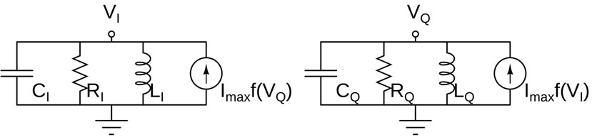
Figure 1. Simplified adopted model for pulsed bias phase and quadrature harmonic oscillator.
pulse is applied to OSC_Q. Such pulse corresponds to a negative half-wave for driven oscillator OSC_Q that becomes delayed of  with respect to driver oscillator OSC_I. In the following calculations we shall always assume the sign “-” for current pulse in OSC_Q.
3. Proof of Quadrature Mode Stability
Since the pulses arise at the crossing of a threshold equal to the common mode voltage of the oscillators, subsequent pulses can be assumed to impinge in two different semi-periods of the oscillation with opposite sign. It can be shown that, in a stable condition, the symmetric scheduling of the pulses leads to the symmetry of the two semi-periods of oscillation. Nevertheless, in order to concentrate our effort on the eigenvector extraction, we propose to adopt semi-periods symmetry as a preliminary assumption. Once the first eigenvector and thus the large signal dynamic will be calculated also the preliminary assumption will be proved. In the following analytical derivations semi-periods symmetry will be formalized as the reflection conditions on the eigenvectors space state.
3.1. First Eigenvector Extraction
As can be easily derived form the adopted model, the evolution of any state variation is a sinusoidal damped function of pulsation  In time intervals when the pulse generators are not active, following RLC system equations, eigenvectors can be described by
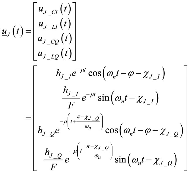 (2)
(2)
where subscripts 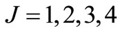 refer to the relative eigenvector number.
  and
and  are unknown eigenvector amplitudes,
  and
and  are the unknown phase displacements between eigenvector components in the two resonators. The
  factor accounts for the ratio between currents and voltages whereas
  factor accounts for relative phase between currents and voltages in a resonator and are given respectively by
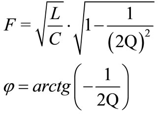 (3)
(3)
For the sake of calculation simplicity in (2) we define  as the amplitude of components related to OSC_Q at
  rather than at
 . We recall that in a stable oscillator always exists a “first” eigenvector with unitary eigenvalue and with components tangent to the space state orbit. This property makes first eigenvector behavior directly related to the oscillator state. E.g. the threshold crossing which triggers the bias current pulse can be indicated either in term of eigenvector components or of oscillator state. In the two oscillators the threshold is indeed crossed as the capacitance voltage zeroes, i.e. when current component of eigenvector is null
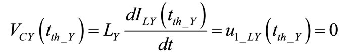 . (4)
. (4)
We assume for the first eigenvector . Since eigenvectors components can always be defined by a proportionality constant, we choose to fix
  with no loss of generality. Similarly we assume the threshold of OSC_I is crossed at
  and for
 . We recall once more that the value of the eigenvalue of first eigenvector must be one. This aspect brings to four the number of independent conditions on eigenvector components. We notice that Equations (2) contain only two unknowns in front of four conditions. The two exceeding conditions indeed will lead to determination of both oscillation period and amplitude.
At this point we must introduce the basic assumption that if  is short enough compared to actual oscillation period T, the overall effect of the current pulse can be approximated with a drop in current components of eigenvectors. In [6] we showed that current drop has the general form
 . (5)
. (5)
The sign of current drops depends upon the sign of capacitor voltage derivative and eigenvector amplitude of the driven oscillator at threshold crossing and on the quadrature sign chosen in Equation (1). Resulting current drops are sketched in Figure 2 by thick arrows for a semi-period. Due to circuit loss  currents and voltages components in resonators are not exactly in quadrature, then current drops may produce both amplitude variations and phase shifts of the orbit. In Figure 2 phase shifts are respectively indicated as
  and
and  for the two oscillators.
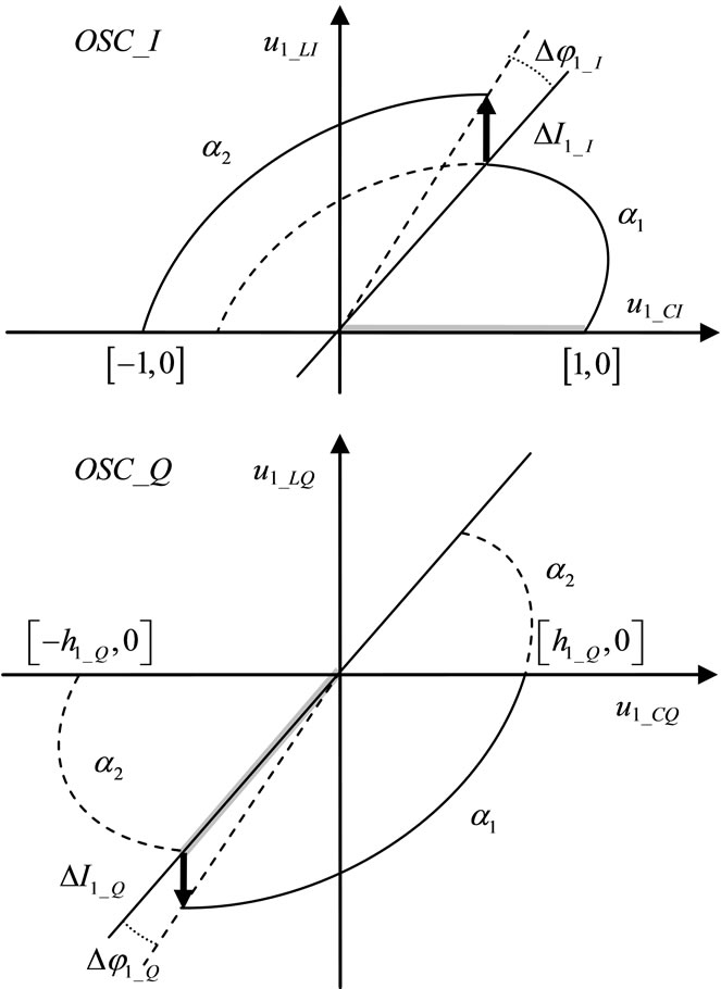
Figure 2. Sketch of evolution of first eigenvector subdivided into OSC_I and OSC_Q plane components. Thick gray line indicates the eigenvector at t = 0.
As previously indicated, under semi-periods symmetry we impose the reflection conditions: after a semi-period each component of the first eigenvector must return to the initial value changed in sign. For the other eigenvectors the conditions will impose each component to reach the initial value times the square root of the eigenvalue changed in sign. Using expressions (2) the reflection conditions can be written as in Equations (6). Before we develop such conditions the evolution along a
 . (6)
. (6)
semi-period must be analytically expressed including the drops induced by pulses. This result can be achieved combining damped evolutions (following RLC system equations) and amplitude and phase shifts due to bias pulses.
We define as  the phase evolution in (2) between application of the bias pulse to OSC_Q resonator and the time instant when its current component,
  , zeroes (0 V threshold crossing by OSC_Q voltage component). We define as
  the phase change between the application of the bias pulse to OSC_I resonator and the instant when its current component,
  , zeroes (0V threshold crossing by OSC_I voltage component).
In [6] the effect of the current pulse is represented as the drop to an equivalent damped sinusoidal evolution always with origin in  but with a different amplitude and an additional phase shift.
First pulse is applied at  to OSC_Q resonator giving rise to phase shift
 . (7)
. (7)
After a damped evolution by a  phase,
  (the OSC_Q threshold) is crossed and a second current pulse is applied this time to OSC_I. The second induced phase shift
  retains memory of former phase shift
  resulting in
 . (8)
. (8)
A further phase evolution of α2 closes the semi-period. Since damped evolution of the two oscillators is identical in both semi-period, total phase evolution must equalize. We may thus write the reflection condition as
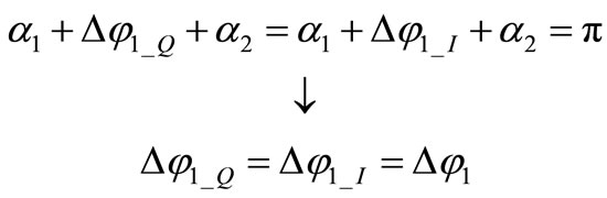 , (9)
, (9)
i.e. the two phase shifts must be equal.
Drop  is dependent on the amplitude
  which is still an unknown. In order not to run through an intricate calculation we now attempt a by inspection solution (requiring a later verification). Basing again on symmetry we assume
 . (10)
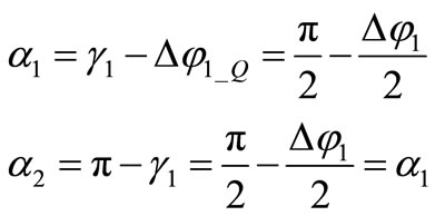
With this assumption and inserting (7)-(8) into condition (9) the expression can be solved equating the arguments of cosine functions
 . (11)
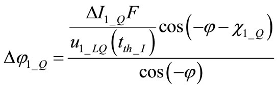
Using (11) in (6) an implicit form for  phase shift is obtained
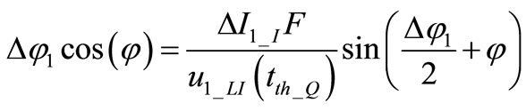 (12)
(12)
which needs to be solved for .
.
We notice that  is well approximated with resonator quality factor just greater then few unities. In the simplified case of
  expression (11) is verified only for
 . This assumption implies
  , i.e. the oscillation period is equal to the natural period of damped RLC resonator. The assumption would also lead to state that
 . In sections 3.2 and 3.3 we are going to perform further calculations on remaining eigenvectors under this particular assumption. Then in section 5 this approximation will be verified through comparison with a dedicated Matlab simulator.
If  we may assume
  in (2) and this ensures that OSC_Q is delayed with respect to OSC_I, thus confirming the effect of signs choice in (1).
Beside these approximations we further use (10) and the reflection conditions to obtain
 . (13)
From (13) we may infer that the two oscillators are intrinsically in quadrature, since the bias pulse generated at the 0V crossing of one of the two resonators is applied at the center of two identical time evolutions between the two bias pulses applied to the other resonator. This property is independent from resonators losses. The oscillation period can indeed be written as
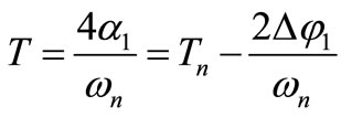 . (14)
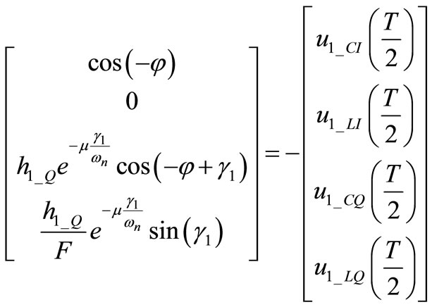
It is possible now to express the reflection conditions (6) in a compact form. Being ensured the parallelism of the eigenvector at  by (9), we may impose the condition only to one component of eigenvector. If we consider
  its value must be equal to current state component at time origin changed in sign
 . (15)
Equation (15) can be solved for  obtaining
 (16)
(16)
Since expression (16) has still two unknowns ( and
and ) it must be solved in conjunction with evolution of OSC_I components. We may calculate the evolution of
  at
at  just after the current drop is added by the bias pulse (superscript ‘+’ indicates in the limit from the right). In particular
  can be expressed through (5) at a time instant
  when the OSC_Q component can be easily calculated using reflection condition as
 . We hence obtain
 . (17)
After a further evolution of  the
the  zeroes. Reflection conditions can now be imposed on the voltage component
 (18)
(18)
to solve again for
 . (19)
We immediately point out that Equations (16) and (19) can be verified simultaneously only if . A straightforward consequence is
 (20)
(20)
Equal oscillation amplitudes for both resonators verify the assumption (10) of equal amplitudes for current drops. This ensures the correctness of the entire calculation. From this statement and considering that also the amplitude of oscillation is a damped sinusoidal function its amplitude can be derived as
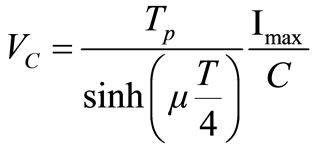 . (21)
As anticipated at the beginning of this section the conditions on the first eigenvector lead to the determination of oscillation amplitude and oscillation period. The existence of a fixed oscillation amplitude ensures also stability of system.
3.2. Extraction of Second and Third Eigenvectors
The second eigenvector can be expressed through (2) with . Again
  and
and  are unknown eigenvectors amplitudes,
  and
and  are the unknown phase displacements between eigenvector components in the two resonators.
We perform a normalization on amplitudes assuming . Since second eigenvector cannot be related to the oscillator state evolution, the only additional condition we may impose is the independence from the first one. We recall we are going again to perform the calculation under the particular assumption that
  (which corresponds to assume
 ), i.e. a damped sinusoidal evolution must cover a phase of
  in a semiperiod.
We combine the extractions of second and third eigenvectors since we may demonstrate that both eigenvectors are related to a unique Floquet eigenvalue with algebraic multiplicity equal to two.
Pulses positions are fixed by the oscillator state. We individuated at  a first current pulse is applied to OSC_Q whereas at
  the second current pulse (in first half of period) is applied to OSC_I.
With the adopted assumptions we obtained  , thus at
  the first eigenvector has the OSC_Q components in the {I} current axis direction and the OSC_I in the {V} voltage axis direction.
In order to preserve geometric multiplicity equal to two, second and third eigenvector must be independent and this requires them to have at  for OSC_Q at least a finite component in the {V} direction and for OSC_I a finite component in the {I} direction.
In addition we must notice that, as in first eigenvector, the phase steps due to bias current pulses must be null to ensure that in  a total phase evolution
  is achieved. Damped sinusoidal evolution (which is equal in all the eigenvectors) is already
  and no additional phase can be added.
Referring again to Figure 1, a null phase step can be achieved only for two conditions:
1) if the eigenvector is in the {I} current direction at instant of application of the pulse, but this is not possible for the independence condition;
2) if the current drops discontinuities induced by the bias pulses are null.
As demonstrated in [6] this can be achieved only if the OSC_I voltage components of eigenvectors is null at  and if the OSC_Q voltage components is null at
 .
.
Imposing these two conditions in (2) we immediately obtain
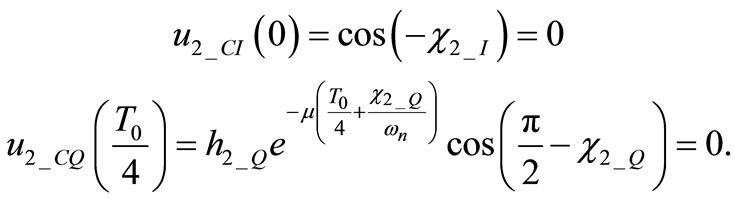 (22)
(22)
Hence it must be verified that  and
and .
.
Without any current drop the eigenvector amplitude exponentially decreases with the natural  damping of the system. There is no further condition to be applied in order to calculate the unknown amplitude
 . This means that reflection conditions on second and third eigenvectors are satisfied for any vectors laying in the plane
  where
where , i.e. that there are two independent eigenvectors with the same eigenvalue:
 . (23)
With no loss of generality we may thus assume  and
and .
.
3.3. Extraction of Fourth Eigenvector
The fourth eigenvector can be expressed through (2) with J = 4. Again  and
and  are unknown eigenvectors amplitudes,
  and
and  are the unknown phase displacements between eigenvector components in the two resonators.
Fourth eigenvector must be independent from all the formerly calculated ,
,  , and
, and .
.
We recall that with approximation  the phase propagation of both OSC_I and OSC_Q amounts in total to
 . Thus also
  must have null values of phase steps. This condition occurs if one of the following two conditions is satisfied:
1)  and
and . Null values of voltage displacement components at threshold crossing corresponding to null current drops, but this condition is completely dependent on eigenvectors
  and
and ;
;
2)  and
and . Eigenvector is parallel to current drops at the time of thresholds crossings thus giving rise to null phase steps. The condition with sign “+” is that of
 .
.
This means we must choose the condition b) with sign “-”. With no loss of generality we fix  then we write at
  the independence condition among the four eigenvectors
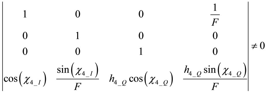 . (24)
For  and
and  we obtain
 (25)
(25)
which is satisfied for any positive value of  The fourth eigenvector evolution is reported in Figure 3 Reported current drops follow the sign imposed by condition (5) as chosen in (1). This make fourth eigenvector components in OSC_Q to be in advance. Change of the eigenvector components sign determines change of sign of current drops contributions to OSC_I. A decrease of eigenvector amplitude is then found in both resonators components.
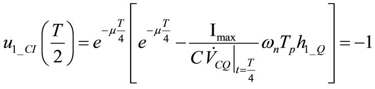
Being ensured the parallelism of the eigenvector at 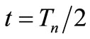 and
and  for (9) we may impose the reflection conditions only to one component: after a semi-period evolution any eigenvector component must reach a value which is the square root of
  times its values at
  changed in sign. We follow the calculation performed for the first eigenvector. For OSC_Q at
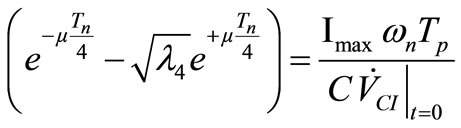
  we have
 (26)
(26)
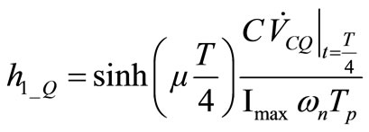
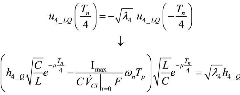
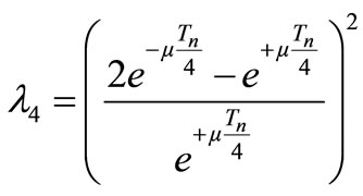
Equation (26) can be solved for h4_Q obtaining
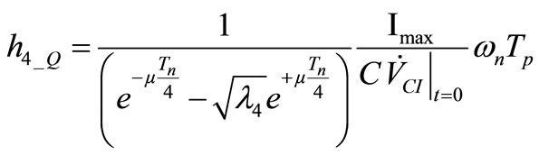 . (27)
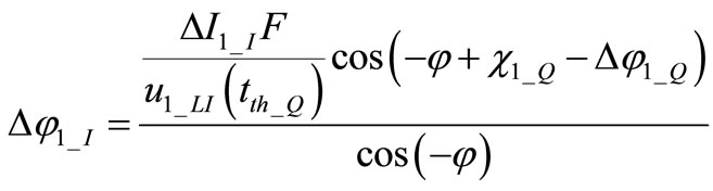
For OSC_I we must first consider the evolution of
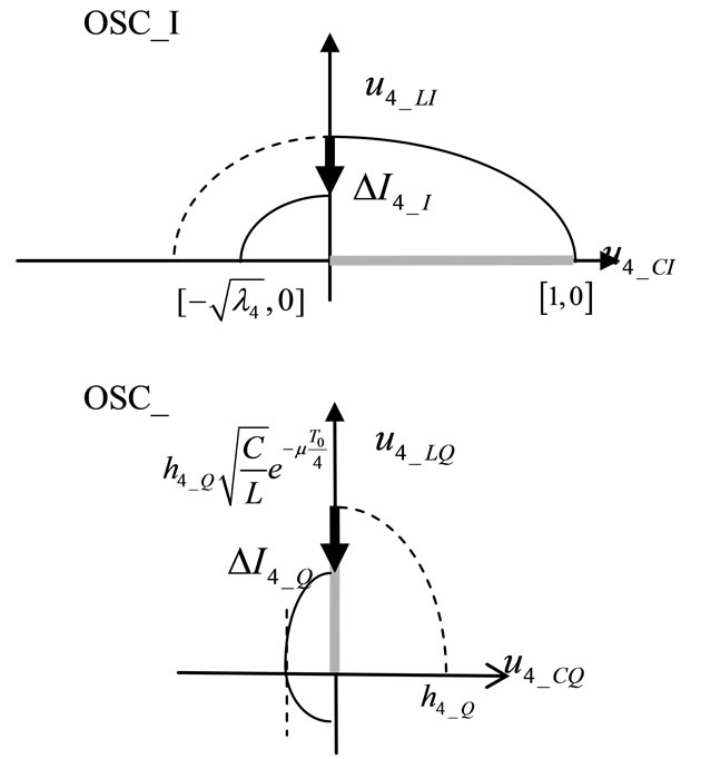
Figure 3. Sketch of evolution of fourth eigenvector subdivided into OSC_I and OSC_Q plane components. The approximation φ = 0 is assumed. Thick gray line indicate the eigenvector at t = 0.
 at
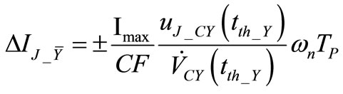
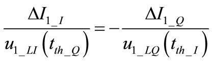
at  where the current drop is added due to the bias pulse. ΔI1_I can be expressed through (5). Pulse on OSC_I depends on the amplitude
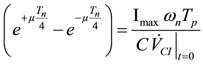
  The reflection condition on OSC_I is written as
 (28)
(28)
Equation (28) needs to be solved again for 
 . (29)
We immediately point out that Equations (27) and (29) can be verified simultaneously only if  h4_Q = 1/h4_Q = 1.
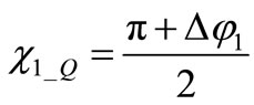
It remains the calculation of . Recalling that the reflection condition can be written as
 (30)
(30)
and that from the first eigenvector assuming  we know that
 , (31)
we finally obtain
 . (32)
4. Noise Projections and Zero Projection Times
Noise introduced by the bias pulse generators and from parasitic resistances projects onto the eigenvectors and evolves following the eigenvalues damping in time. The relationship between these projections and the overall phase noise has been extensively described elsewhere [7- 10]. We can briefly state that the lower is the integral along the period of the variance of the projection of noise contributions onto the first eigenvector, the lower is the  component of phase noise close to the fundamental. We can thus try to evaluate the contribution of projection of the two cited main noise sources.
We define as Zero Projection Times (ZPT) the instants of the limit cycle when noise introduced by a generic source does not project onto the first eigenvector. This is particularly important for the bias current generators which should be switched on preferably around a ZPT. As we have seen along the calculation, eigenvectors evolution is strictly related to the pulse position. Then eigenvectors and pulses cannot be defined independently. Actually we may show that in the presented architecture ZPTs in the optimal position correspond to the time of application of the bias pulses.
We recall at  and
and  current pulses are found on OSC_Q. We model a normalized white Gaussian process as two additional parallel and independent current sources (one source per resonator). Such noisy process generates a state variation in the direction
  for OSC_Q. This variation is in the plane of eigenvectors
  and
and  and orthogonal to
 . Thus it implies a null projection onto the first eigenvector.
At  and
and  the pulse is in OSC_I. In this case the process generates a state variation in the direction
 . Eigenvectors
  and
and  after a phase evolution of
  still span a plane which contains this vector and thus remains orthogonal to
 . This implies again a null projection onto the first eigenvector.
Hence we state that ZPTs correspond exactly to the bias pulses application instants. This aspect represents the main property of the presented architecture, since it ensures that noise introduced by the bias does not project onto the phase noise close to the fundamental. In section 5 simulation will confirm this peculiar behavior.
A second relevant property can be inferred form the eigenvectors description. Further relevant noise sources come from parasitic resistances of the resonators. These noise contributions exist all along the period (stationary source) and are not time limited as the bias noise (ciclostationary source). In this case it is essential that the projections occur onto orthogonal eigenvectors. Indeed non orthogonal orientation of the eigenvectors would give rise to an enlargement of the stationary noise source projections. Since any projection on  is not decreased by the exponential damping due to the eigenvalue
 , non orthogonal eigenvectors reflect unavoidably in a phase noise enhancement.
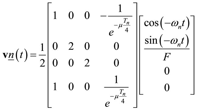
We showed in [6] minimization of the integral of a stationary variance projected onto the first eigenvector occurs under the condition of orthogonal eigenvectors. We may adapt this result to the case of noise vector  generated by the parasitic resistance in one of the two resonant circuit and verify the condition of minimum projection in a period. We extract in (33) the left eigenvectors v at
  inverting the right eigenvectors matrix u derived from former results. The components of first eigenvector are normalized to one in order to make more explicit the result of projection even if a normalization is not necessary. Being uncorrelated, noise contributions from the two resonators can be considered independently. Noise has a fixed direction while each component of the eigenvectors rotates with pulsation ωn as given in Equation (2). For the sake of simplicity we may change the reference assuming new axes solid with the eigenvectors, so that noise components appear as a rotating
  vector. At every time instant the total energy from the two noise components is maintained constant.
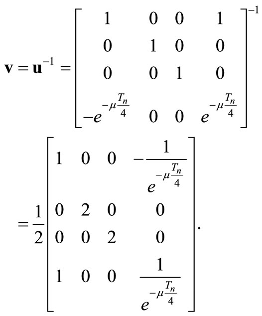 (33)
(33)
It can be easily verified from (34) that each noise generator arising from one single resonant circuit always results projected only along two state components and that the two directions are orthogonal. E.g noise from OSC_I is projected along  and
and  . It is worth to notice that the projections onto first and fourth eigenvectors are identical with coefficient 1/2 while there is a projection on eigenvector
  with coefficient 1.
 . (34)
Vice versa contribution from noise in OSC_Q results projected along two constant orthogonal directions  and
and . Projections onto the first and fourth eigenvectors are again identical with coefficient 1/2 while this time we have projection on eigenvector
  with coefficient 1.
Having assumed noise generators independent in the two resonators, the variances of projections onto first and fourth eigenvectors can be summed. Hence due to the coefficient on the amplitudes, the total variance of the projection on first eigenvector results to be 1/2 of the value obtainable in a single resonator. In other words and to our knowledge, we obtained the first analytical demonstration of effective reduction of noise projection onto the first eigenvector due to phase and quadrature coupling of oscillators.
5. Simulation Results and Discussion
The approximation introduced in the former calculation requires a numerical verification. This is done in the present section by the use of a piece-wise linear integration method that gives an exact evaluation of the system reported in Figure 1.
The simulation method adopts in particular Interface Matrices for the description of the state variation at the current pulse discontinuities [11]. This method allows to extract eigenvectors and eigenvalues with high accuracy. For the simulation we choose two given values for capacitances and inductances respectively  and
and  producing ideal resonance at
  even if the developed theory is not frequency dependent. We fix also the total charge of a single current pulse in
 . In Figure 4. the eigenvalues for the pulsed bias phase and quadrature oscillator are reported in both calculated (continuous traces) and simulated (dotted traces) cases as a function of resonators quality factor. It can be observed a very good match between calculated and simulated
  (error always <1%) whereas calculated
  is underestimated with respect to the simulated one (error <5% for
 ). Underestimation is due to
  assumption which leads to higher error in determination of expression (32).
In Figure 5. we report the simulated projections of  and
and  noise perturbation vectors onto the first eigenvector in case
 . Such noise vectors describe both the effect of bias current generator and parasitic resistance noise respectively of
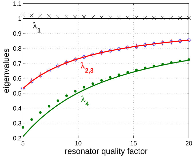
Figure 4. Eigenvalues of proposed oscillator as a function of resonator quality factor. In continue traces (black line is λ1, red line are λ2,3 and green line is λ4) the analytical expressions are plotted whereas in dotted traces (black “x” is λ1, red “+” and blue “o” are respectively λ2 and λ3 and green solid “o” is λ4) the results of simulator are reported.
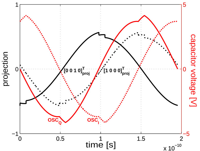
Figure 5. Simulated projections of [1 0 0 0]T (black dotted trace) and of [0 0 1 0] T (black continuous trace) onto first eigenvector  and related capacitors voltages (OSC_I in red dotted trace, OSC_Q in red continuous trace) of resonators in time of proposed oscillator for Q = 10.
the two resonators. The phase and quadrature oscillation of capacitances voltages is also reported in the figure. The evident presence of discontinuities on voltage waveforms induced by bias pulsed currents allows to verify that null projections correspond exactly to the pulses injected in relative resonators. We remark that maximum projection is 1/2 corresponding to the normalized noise charge injected onto the  capacitor. Absence of any increase above value 1/2 of projection is the effect of the eigenvectors orthogonality.
Finally in Figure 6, we report the value of the oscillation period and amplitude in calculated (continuous traces) and simulated (dotted traces) as a function of the resonators quality factor. In this evaluation the calculated expressions present a maximum of 1.8% error for period and of 11.8% error for amplitude at low quality factor value compared to simulated results. Both errors become <1% as Q increases above 10.
6. Concluding Remarks
We presented the full analytical description of a new class of pulsed bias phase-quadrature oscillators. Introducing a new methodology entirely based on system state Floquet eigenvectors we proved existence and stability of the quadrature mode and derived a consistent noise analysis. We pointed out a direct relationship between circuit parameters and the exclusive noise performances of the architecture. In particular we highlighted the intrinsic orthogonal behavior of the coupled oscillators, the possibility to obtain a minimum projection of noise introduced by the bias pulse on first eigenvector and finally the intrinsic orthogonality of the eigenvectors. We furthermore demonstrated that such properties ensure minimization of phase noise contributions from both the
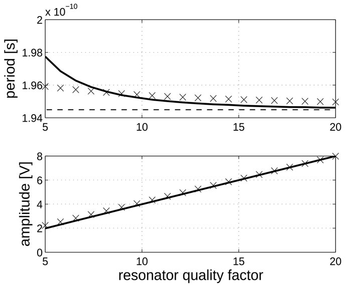
Figure 6. Period and amplitude of oscillation of proposed oscillator as a function of resonator quality factor. In continue traces the analytical expressions are plotted whereas in dotted “x” traces the results of simulator are reported. The dashed line in top subfigure represents period of resonator with no loss.
parasitic resistances and the eventual active devices performing the pulsed energy restore. Exploited properties should be common to the entire class of phase-quadrature oscillators with fixed duration current bias pulses. Nevertheless the analysis of a practical electronic realization of the architecture and its evaluation requires and deserves a dedicated work.
REFERENCES
- P. Andreani and X. Wang, “On the Phase-Noise and Phase-Error Performances of Multiphase LC CMOS VCOs,” IEEE Journal of Solid State Circuits, Vol. 39, No. 11, 2004, pp. 1883-1893. doi:10.1109/JSSC.2004.835828
- S. Perticaroli and F. Palma, “Phase and Quadrature Pulsed Bias LC-CMOS VCO,” SCIRP Circuit and Systems, Vol. 2, No. 1, 2011, pp. 18-24. doi:10.4236/cs.2011.21004
- T. H. Lee and A. Hajimiri, “Oscillator Phase Noise: A Tutorial,” IEEE Journal of Solid-State Circuits, Vol. 35, No. 6, 2000, pp. 326-336. doi:10.1109/4.826814
- A. Demir, “Floquet Theory and Non-Linear Perturbation Analysis for Oscillators with Differential-Algebraic Equations,” International Journal of Circuit and Theory Applications, Vol. 28, No. 2, 2000, pp. 163-185. doi:10.1002/(SICI)1097-007X(200003/04)28:2<163::AID-CTA101>3.0.CO;2-K
- G. J. Coram, “A Simple 2-D Oscillator to Determine the Correct Decomposition of Perturbations into Amplitude and Phase Noise,” IEEE Transactions on Circuits and Systems—I: Fundamental Theory and Applications, Vol. 48, No. 7, 2001, pp. 896-898. doi:10.1109/81.933331
- S. Perticaroli and F. Palma, “Design Criteria Based on Floquet Eigenvectors for the Class of LC-CMOS Pulsed Bias Oscillators,” Microelectronics Journal, 2011, Article in Press. doi:10.1016/j.mejo.2011.07.018
- F. X. Kaertner, “Analysis of White and f-α Noise in Oscillators,” International Journal of Circuit and Theory Applications, Vol. 18, No. 5, 1990, pp. 485-519. doi:10.1002/cta.4490180505
- A. Demir, A. Mehrotra and J. S. Roychowdhury, “Phase Noise in Oscillators: A Unifying Theory and Numerical Methods for Characterization,” IEEE Transactions on Circuits and Systems—I: Fundamental Theory and Applications, Vol. 47, No. 5, 2000, pp. 655-674. doi:10.1109/81.847872
- A. Carbone, A. Brambilla and F. Palma, “Using Floquet Eigenvectors in the Design of Electronic Oscillators,” Emerging Technologies: Circuits and Systems for 4G Mobile Wireless Communications, 2005. ETW’05. 2005 IEEE 7th CAS Symposium, 23-24 June 2005, pp. 100-103. doi:10.1109/EMRTW.2005.195690
- A. Carbone and F. Palma, “Considering Orbital Deviations on the Evaluation of Power Density Spectrum of Oscillators,” IEEE Transactions on Circuits and Systems —II: Express Briefs, Vol. 53, No. 6, 2006, pp. 438-442. doi:10.1109/TCSII.2006.873527
- A. Carbone and F. Palma, “Discontinuity Correction in Piecewise-Linear Models of Oscillators for Phase Noise Characterization,” International Journal of Circuit Theory and Applications, Vol. 35, No. 1, 2007, pp. 93-104.