Journal of Modern Physics
Vol.5 No.9(2014), Article ID:47366,16 pages
DOI:10.4236/jmp.2014.59092
The Light as Composed of Longitudinal-Extended Elastic Particles Obeying to the Laws of Newtonian Mechanics
Alfredo Bacchieri
University of Bologna, Bologna, Italy
Email: abacchieri@libero.it
Copyright © 2014 by author and Scientific Research Publishing Inc.
This work is licensed under the Creative Commons Attribution International License (CC BY).
http://creativecommons.org/licenses/by/4.0/


Received 16 April 2014; revised 12 May 2014; accepted 7 June 2014
ABSTRACT
It is shown that the speed of longitudinal-extended elastic particles, emitted during an emission time T by a source S at speed u (escape speed toward the infinity due to all the masses in space), is invariant for any Observer, under the Newtonian mechanics laws. It is also shown that a cosmological reason implies the light as composed of such particles moving at speed u (function of the total gravitational potential). Compliance of c with Newtonian mechanics is shown for Doppler effect, Harvard tower experiment, gravitational red shift and time dilation, highlighting, for each of these subjects, the differences versus the relativity.
Keywords: Escape Speed, Harvard Tower Experiment, Time Dilation, Redshift, Doppler Effect, Compton Effect

1. Introduction
Here we present a solution, in accordance to the Newtonian mechanics, to the apparent constancy of c, based on following assumptions:
1) Gravity fields fixed to their related masses (intending that each field is moving together with its generating mass).
2) Finite mass of the universe, implying a finite value of U (total gravitational potential) and therefore of u (escape speed from the universe due to all the masses in space).
3) Light composed of longitudinal-extended elastic particles (as defined on §4) moving at speed c = u. This equality is supported by a cosmological reason, see §2.
On above bases (including, needless to say, Newton’s absolute time and space) we find:
a) The relation between u (total escape speed) and U (total gravitational potential), giving to the speed of light the cosmological reason of its value.
b) On Earth, the variation of u, (and therefore of c as per assumption III), due to the variation of U (mainly caused by the variable distance Earth-Sun) is, during one year, Δu (=Δc) ≤ ±0.05 m×s-1, hence within the accuracy of the measured value of c.
c) The invariance of the measure of c for any Reference frame under the Newtonian mechanics laws.
d) The longitudinal, generic and transverse Doppler effect for longitudinal-extended elastic particles, as defined, and their physical characterization.
e) As for the Harvard tower experiment [1] -[3] , regarding the variation of frequency (or wavelength) between a source (of gamma rays) and an absorber at different height, our relations give a shift equal to the observed and also predicted by the Relativity. Anyhow, with the source on the base (of the tower) the light arriving to the top has, as for the GR, a lower frequency, whereas on our bases, is the length of our particles which decreases (together with c); on the contrary, with source on the top, GR predicts an increase of the frequency of the light arrived to the base, whereas we show that, during the same path (top-base), is the length of these particles which increases (together with c), giving a red shift. Moreover, as for the value of the compensating speed source-absorber, (necessary to restore their resonance), we point out that the experiment did not give any clear indication about the effective direction of this speed. Indeed, scope of that experiment was to “establish the validity of the predicted gravitational red shift” [2] , hence the only value of this speed was taken in consideration; here, on §6, we show that, on our bases, the effective direction of this speed is contrary in both cases (source on top or base), to the one predicted (but not verified) by the Relativity.
f) As for the gravitational time dilation, on §6, it is shown that taking a source (of light) in altitude, it yields a negative variation of c as well as a negative variation of the frequency n inducing atomic clocks to run faster; moreover, through our Equation (29) regarding a source circling (around the Earth), we obtain, see (46), the exact variation of the ticking time of GPS system.
g) As for high red shifts related to far sources, we show that, disregarding the relative motion Earth-source, they depend on the increase of c (as well as the increase of the length of the said “longitudinal-extended elastic particles”) during the path of light toward higher (in absolute value) potential; on §7, Table 1, we give the values of c (on these far sources) related to the observed red shifts.
h) Our Equation (17), (regarding our Doppler effect for the light), applied to the Compton effect (indubitable Doppler effect), gives, see Appendix A, the Compton equation, which cannot be obtained through the relativistic Doppler effect equations.
2. Total Escape Speed (from a Point toward the Infinity) Due to All the Masses in Space
As known, considering in space one only mass M (regarded as a point-like), the gravitational
potential U acting on a particle having mass m = M, assuming U¥
= 0, with s the distance M-m, is U = −MG/s; this relation, according to our
first assumption (I), is always valid in spite of any reciprocal motion between
M and m. The related Conservation of Energy (CoE), E = U + K, (where K =
 represents the unitary, i.e. for unit of masskinetic energy of our particle arriving
from the infinity, where u¥ = 0), for
E = 0 gives U = −K, leading to
represents the unitary, i.e. for unit of masskinetic energy of our particle arriving
from the infinity, where u¥ = 0), for
E = 0 gives U = −K, leading to
 (1)
(1)
which is a scalar, (called escape speed), representing (in the considered point) the value of the velocity u, any massive particle, under a potential U, needs to reach the infinity, so u (escape velocity)must be referred to M.
Considering now two masses M1 and M2, having, at a given time, distances s1 and s2 from a considered point (we may call it Emission point Ep), the potential U1,2 in Ep becomes
 (2)
(2)
Now, the escape speed from two masses can be written
 (3)
(3)
which is the value, in the considered point Ep of the (escape) velocity u1,2 which has to be referred (at the considered time), to the point, we may call it Centre of potential (Cp), where |U1,2| has the max value. Then, as
 and
and
 we also get
 (4)
(4)
therefore the escape speed due to all the n masses in space becomes
 (5)
(5)
with
 the universe mass,
 the total gravitational potential in the considered
point Ep, and where u (function of U in Ep) can be called
as total escape speed (toward the infinity), while the escape velocity u is referred
to the centre Cp. Indeed, any unitary massive particle during its path
toward the infinity, has to comply with the CoE, U + K = 0, where K =
the total gravitational potential in the considered
point Ep, and where u (function of U in Ep) can be called
as total escape speed (toward the infinity), while the escape velocity u is referred
to the centre Cp. Indeed, any unitary massive particle during its path
toward the infinity, has to comply with the CoE, U + K = 0, where K =
 giving to this particle a speed u
(which depends on the location of the source) and yielding, for all the masses, the total energy equal to zero [Compliance of light with above relation E = U + K, is shown on Appendix B].
We assume now the equality c = u, hereafter supported by the estimated mass of universe and also by a cosmological reason: in fact, if c > u the energy of light will be lost forever and furthermore the observable masses, following the always increasing mass of light going toward the infinity, will also tend to the infinity moving away from each other. On the contrary, if c < u, all the masses in space (having speed lower than u), will tend to a gravitational collapse, whereas for c = u, the mass of light, tending to the infinity in an unlimited time, will avoid the two said events (collapse or dispersion).
Now the mass of universe, by some authors, is estimated [4]
-[6] to be
 kg; the same order of magnitude is given through the number (
 ) of observable stars
[7] [8] , and since
from Earth the distribution of the masses appears to be homogeneous and isotropic,
under our assumption U¥ = 0, we may assume
their density as decreasing toward the infinity like a function ρ = ρce−as
with
) of observable stars
[7] [8] , and since
from Earth the distribution of the masses appears to be homogeneous and isotropic,
under our assumption U¥ = 0, we may assume
their density as decreasing toward the infinity like a function ρ = ρce−as
with
 kg/m3 the critical
density [9] . So the mass of universe can be written
kg/m3 the critical
density [9] . So the mass of universe can be written
 (6)
(6)
yielding
 (7)
(7)
On Earth, the variation of potential due to an increase of the distance ds, can be written as dU = −dmG/s where dm = ρ4πs2ds with ρ = ρce−as, hence the potential on Earth becomes
 (8)
(8)
Now, according to (5), on Earth it is
 (9)
(9)
Therefore, on Earth, uo = co, so that
 and, in general we may argue
 (10)
(10)
The equality c = u, which implies the massiveness of light, means that, along any free path, the speed of light only depends on the value of the potential along that path.
[As for the relation , the Harvard tower
experiment has shown that the fractional change in energy
, the Harvard tower
experiment has shown that the fractional change in energy
(of light) is given by δE/E = −gh/c2, and since the term gh is the variation of potential from the ground to the height h, we may guess that c2 has to be related to the total gravitational potential, as also shown on §6].
3. Annual Variation, on Earth, of the Total Escape Speed
On Earth a small variation of the total escape speed uo, from (9), can be written as
 (11)
(11)
where ΔU is the variation of the total potential on Earth, mainly due to the variable distance Earth-Sun.
So considering the eccentricity e (=0.0167) of Earth’s orbit around the Sun, between their average distance d (=1.5 ´ 1011 m) and their shortest distance (Perihelion) p = (1 – e)d, and with u0 = 3 ´ 108 m×s-1, the (11) gives
 (12)
(12)
with Δue the variation of u due to Earth’s orbit eccentricity, ΔUS
the variation of potential on Earth due to Sun between the two said distances, with
MS the mass of Sun. Hence from Aphelion to Perihelion, one should find
ΔuAP (=ΔcAP) = +0.10 m×s-1and we note that
this variation is compatible with the accuracy of the measured value of c = 299792458
m×s-1. Due to Earth’s rotation, there is also a daily variation which,
from midnight to noon, is of the order of ; so, on Earth, uo
is practically constant during one year, as it is for the measurements of the speed
of light.
; so, on Earth, uo
is practically constant during one year, as it is for the measurements of the speed
of light.
4. Invariance of c for a Particular Particle, Here Defined, and Related Doppler Effect
Here we show that the Galileo’s velocities composition law, (related to point-particles), cannot be correctly applied to a particle, (hereafter called photon), defined as follows:
“Longitudinally-extended, elastic non divisible particle emitted at speed u by a source during an emission time T, and moving along one ray (continuous succession of photons), where two consecutive photons cannot be separated along a free path (constraint of non separation)”.
Of course, more photons emitted during an emission time T need an equal number of rays.
Calling front and tail the extremities of a photon, the constraint of non separation implies that, along a ray, any tail corresponds to the front of the next photon.
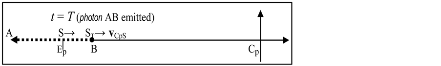
Referring to Figure 1(a) (where Ep is the location of S at t = 0 and ST its location at t = T), since the escape velocity c (=u) of an emitted photon (AB) is referred to the Centre of potential Cp, during its emission time (0 ≤ t ≤ T), the term vCpA = u should appear as the velocity of its front (A) from Cp.
The source S may have a velocity vCpS from Cp, thus writing vCpA = vCpS+ vSA we should find vSA = u − vCpS; this means that each photon emitted around the source should have a length λ' = |vSAT| = |(u − vCpS)|T depending on vCpS, but this is contrary to the experience showing that if the source is fixed to its initial Emission point Ep (that is the point where S is located at the start of the emission) the emitted photons, referring to Ep, have equal characteristics. Thus, during the emission of a photon, the velocity of its front, (to comply with these equal characteristics), has to be referred to the initial Emission point Ep, therefore, see Figure 1(b), where Ep is our reference frame, as for the front A, for definition, we have
 (13)
(13)
[This condition also allows the whole photon to have a velocity u referred to Cp, as shown on Figure 1(d)].
Now the velocity of the front A, with respect to S, from (13), becomes
 (14)
(14)
and still referring to Figure 1(a), (where ST is the location of S at t = T), should S be fixed to Ep (that is vEpS = 0), the length λ of each photon, after the emission time T, from (14) becomes λ = vSAT = uT, while, in general, it is
 (15)
(15)
where
 is the photon AB emitted with the source in motion from Ep.
Referring now to Figure 1(c), if a generic Observer O is our Reference frame, we can write
 (a)
(a)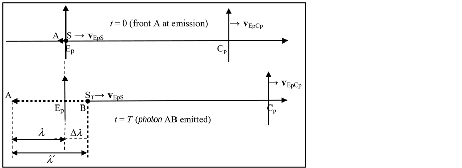 (b)
(b)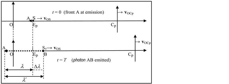 (c)
(c)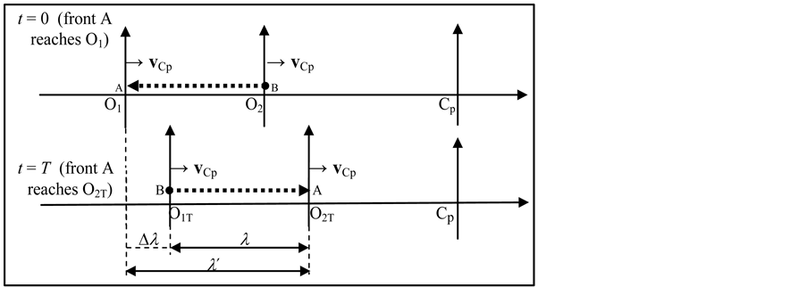 (d)
(d)
Figure 1. (a) Photon AB emitted under the supposed condition vCA = u; (b) Emission of a photon AB referred to the initial Emission point Ep; (c) Emission of a photon AB referred to the generic Observer O; (d) Measurement of the speed of a photon (AB) reflected by O1.
 (16)
(16)
where
 is the photon emitted while the source is in motion, with velocity vOS,
from the Observer, and once more, if vEpS = 0 (S fixed to Ep),
we find λ' = λ = uT (If S is now our Reference frame, and vEpS is the
velocity of S from Ep, we still have the (15)).
is the photon emitted while the source is in motion, with velocity vOS,
from the Observer, and once more, if vEpS = 0 (S fixed to Ep),
we find λ' = λ = uT (If S is now our Reference frame, and vEpS is the
velocity of S from Ep, we still have the (15)).
Thus, after the emission time T, as for a source receding from the front of the considered photon, as in Figure 1(b) (or Figure 1(c)), the length λ' (for any Observer) turns out to be
 (17)
(17)
where v (=|vEpS|) is the speed (referred to Ep) of the source S (along the direction EpS), Δλ (=vT) is the path covered by S during T, and where β = v/u, and we point out that the length λ' may change, along a free path, and under constant potential, only during its emission.
Now, the speed of a point-particle is defined through two Observers, while the speed u' of a photon, because of its variable length during its emission, does not correspond to the speed of any point of it, hence we must consider its length referred to the time T' (transit time) the photon (front to tail)needs to cross one Observer, so it has to be defined
 (18)
(18)
[As for this definition, let us consider a system composed of two balls connected through an elastic thread and let them fall in vertical line: during the fall, each part of the system has different speed, so we define the speed of the whole system according to Equation (18)].
Returning now to Figure 1(c), for the Observer O, the transit time T' of the photon AB is given by the time the front A spend to cover the path λ, that is T(λ/u), plus the time the tail B needs to cover the path ST − EP = Δλ; now, once the photon AB has been emitted (at t = T), the velocity of the front A has to be the same as any other part of the emitted photon, hence the time needed by B to cover the path Δλ is ΔT = vT/u, giving
 (19)
(19)
Now, according to (18), the speed of the photon AB, referred to O, becomes
 (20)
(20)
showing that the speed of photons emitted by a source S is invariant for any Observer, in spite of any speed of S with respect to the Observer [After the emission, each part of the photon has same velocity u, meaning that, during the emission, it is the velocity of its inner part to vary in order to change its length in the given time T].
As for an emitted photon, the measurement of c (through the method d/t) implies its absorption and reflection by an Observer. In this way, the Observer becomes the source of a new photon, with the Observer/Source located in the Emission point Ep, so we may refer to Figure 1(b), with the source fixed in Ep, finding u' = λ/T = u.
[Anyhow, we may obtain the same result (u' = λ'/T' = λ/T = u) as follows:
the measurement of c (through the method d/t) implies two Observers at a constant
relative distance O1O2; on these bases, see
Figure 1(d) where Cp is now our Reference frame, after the reflection
of the photon from O1, at t = T, the path covered by the front A to reach
O2T is given by O1O2T that is λ¢ = λ
+ Δλ where λ is the length of the emitted photon AB and where Δλ = vCpT/c,
with vCp the speed of our frame O1O2 with respect
to Cp, yielding λ' = λ(1 + β) where β = vCp/c. The time needed
by the front A to cover the distance O1O2T is T' = T + Δλ/c
= T(1 + β), thus the measured speed (referred to the two Observers) becomes c' =λ'/T'
= λ/T = c in spite of any velocity of the co-moving Observers O1
O2 with respect to Cp (Anyhow, the Observer
O1 could state, for the front A, a velocity
 different from u, if he could measure such a speed)].
For any Observer, the frequency of photons of the same ray has to be defined as n' = n/t with n the number of photons crossing the Observer during a time t; for t = T' (transit time of one photon), it is n = 1, thus n' = 1/T', so from (19) we get
 (21)
(21)
showing that for v = 0, that is β = 0, we have n' = n, which is also valid if the Observer (O) and the source (S) belongs to different potential: in fact, for O and S at reciprocal rest, the number of photons emitted by S in a unit time has to be equal, in the same time, to the number of them crossing O (like, for instance, the number of balls falling from the top of a tower with respect to an Observer at the tower base), and this implies ns = no.
Now, the Figure 1(c), where a source emits a photon while it is in motion from the Observer O, also represents a longitudinal Doppler effect, which, in general, can be written a
 (22)
(22)
with the sign + for S receding from the Observer, while the sign – is for S approaching it.
Hereafter we get our equations regarding both the generic and the transverse Doppler effect, followed by our relations regarding a source (of light) circling around an Observer.
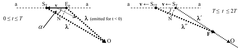
To get a general relation for the Doppler effect, let us consider, see Figure 2(b), referring to the Observer O, a source S, located in Ep (at t < 0), at rest with O. During this time let S emit photons having length λ (=uT) and let EpO = λ. Then, at t = 0, let S start to move from Ep toward ST (reached at t = T), with velocity v (referred to O) along the generic direction a-a. Now, during the path EpST, let S emit a photon λ¢ toward O. (On Figure 2(a), the small arrow inside the triangle EpOST represents the partial λ¢ during its emission.) At t = T (end of emission), according to (16) we have λ¢ = λ ‒ vT, thus the length of λ¢, assuming v = u, so to consider EpO = NO, with EpN ┴ STO, becomes
 (23)
(23)
As for the transit time T', as before, we can write .
.
which can also be obtained considering that the front of λ¢, following the tail of λ (thus directed toward O), takes a time T to reach O from Ep, while the tail of λ¢, emitted in ST, has to cover the path STO = STN + NO, spending the time ΔT = (vTcosα)/u for the path STN, plus the time T for the path NO (equal to EpO for v = u), giving
 (24)
(24)
yielding
 (25)
(25)
thus
 (For an opposite direction of S we get λ' = λ(1 ‒ βcosα) and T' = T(1 ‒
βcosα).
(For an opposite direction of S we get λ' = λ(1 ‒ βcosα) and T' = T(1 ‒
βcosα).
[Ray S2TFO: referring now to Figure 2(b),
if S, between T and 2T, is still moving with same velocity v, the emitted photon
 will have same length as
 , thus its front (at t
= 2T) will reach a point F, (corresponding at the same time to the tail of
, thus its front (at t
= 2T) will reach a point F, (corresponding at the same time to the tail of ), at a distance
 from O, so the ray Source-Observer, at t
= 2T, becomes the line S2TFO].
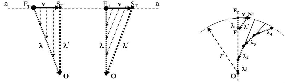
Transverse Doppler effect: referring to Figure 3(a)
left part, where , should S start to move
at t
, should S start to move
at t
= 0 from Ep to ST while emitting the photon , according to (16) we
can write
, according to (16) we
can write
 (valid for S approaching O) (26)
 (a) (b)
Figure 2. Doppler effect for a photon, general case.
 (a) (b)
Figure 3. (a) Transverse Doppler effect; (b) Source circling around the Observer O.
where
 is the length corresponding to STO, while λ corresponds to EpO.
On the contrary, see Figure 3(a) right part (where
the source is receding from the Observer), it will be
is the length corresponding to STO, while λ corresponds to EpO.
On the contrary, see Figure 3(a) right part (where
the source is receding from the Observer), it will be
 (valid for S receding from O) (27)
Then , hence
 .
.
Regarding a source circling around an Observer O, on Figure 3(b) the line EpO represents a succession of photons λ already emitted when S is fixed in Ep, while EpF represents the last of them (or it could represent the last photon emitted by S when reaching Ep). Then, at t = 0 let S start to move from Ep with velocity v toward ST.
Now, because of the constraint of non separation, the front of the first photon
 emitted when S is moving between Ep and ST, has to reach,
in F, the tail of previous photon, so, according to (16) the length of every photon
emitted when S is moving between Ep and ST, has to reach,
in F, the tail of previous photon, so, according to (16) the length of every photon
 (emitted while S is moving along the orbit r) will be
 (28)
(28)
thus
 (29)
(29)
with r the orbit radius, ω the angular speed, giving to any whole photon the speed c' = c.
Figure 3(b) also shows a path (λ1-λ4) of a ray directed toward O (the lines connecting the photons λ2 and λ3 to the orbit give the point where the source is located at the end of their emission).
5. Physical Characterization of These Photons
Now, similarly to a fluid flowing in a pipe (whose kinetic energy is K =
 mv2 with m the mass passing in 1 s)the kinetic
energy of light flowing along one ray (according to our definition, photons are
also massive), has to be expressed with Kc =
mv2 with m the mass passing in 1 s)the kinetic
energy of light flowing along one ray (according to our definition, photons are
also massive), has to be expressed with Kc =
 mc2 with m the mass of the particles
passing in 1 s along one ray. Anyhow, the total energy of light flowing along one
ray is E = mc2 as also proved by the evidences of nuclear reactions like
n + p ® d + γ: indeed, in this reaction [10] , the lost mass, known through mass spectrometers, corresponds
to the value m = E/c2 where E (=hc/λ), (as λ is measured), is also known,
so E = mc2 represents the total energy of light flowing along one ray
(λmeas is obtained [11] through the
value λmeas/(d220) given at pag. 369, where (d220)
is given at page 410).
mc2 with m the mass of the particles
passing in 1 s along one ray. Anyhow, the total energy of light flowing along one
ray is E = mc2 as also proved by the evidences of nuclear reactions like
n + p ® d + γ: indeed, in this reaction [10] , the lost mass, known through mass spectrometers, corresponds
to the value m = E/c2 where E (=hc/λ), (as λ is measured), is also known,
so E = mc2 represents the total energy of light flowing along one ray
(λmeas is obtained [11] through the
value λmeas/(d220) given at pag. 369, where (d220)
is given at page 410).
So, writing E =
 mc2 +
mc2 +
 mc2 we may infer that each of these
particles is provided with an internal energy (Ki =
mc2 we may infer that each of these
particles is provided with an internal energy (Ki =
 mc2) equal to its kinetic energy.
Now, equating mc2 to
mc2) equal to its kinetic energy.
Now, equating mc2 to
 we get
 (30)
(30)
where m written as
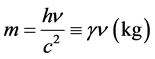 (31)
(31)
is the mass of light, with frequency , passing along one
ray in 1 s, while the constant
, passing along one
ray in 1 s, while the constant
 (32)
(32)
is the mass of light passing along one ray during T, we may call it “mass of one photon”; so one finds
 (33)
(33)
and therefore the Planck’s constant represents the energy of one photon. The energy of these particles passing in 1 s along one ray (energy of one ray of light) can now be written as
 (34)
(34)
On the above bases, the total energy of light emitted by a source is given by nrmc2 with nr the number of rays, and since m is the mass of light passing along one ray in 1 s, this unitary (for unit of time) energy shall be equal to the supplied power P during 1 s, thus nrmc2 = P, hence the total mass lost per second mT (ºnrm) by a source of light becomes
 (35)
(35)
So, for a 1 W lamp, we get mT = P/c2 @ 1.1 ´ 10-17 kg×s-1, while the number nr of rays is
 (36)
(36)
in our case, nr @ 3 ´ 1018 rays. We point out that for
a given power P, the higher is the frequency, the lower is the number of rays, as
shown by (36) written as
 = P/h. The number of photons emitted in 1 s becomes:
 (37)
(37)
which, for P = 1 W, gives nγ = h‒1 (=1.5 ´ 1033 photons/s), so the inverse of Planck constant corresponds to the number of photons emitted in 1 s by a source of unitary power (This great number of photons (having emission time T at speed c) can be regarded as a wave function).
Now the momentum of the photons passing along one ray in 1s, considering their kinetic
energy only, that is Kc =
 mc2, according to Newtonian mechanics
should be written as
mc2, according to Newtonian mechanics
should be written as
 (38)
(38)
but considering both their kinetic and their internal energy, that is E = mc2 we obtain
 (39)
(39)
6. Revisitation of the Harvard Tower Experiment and Time Dilation
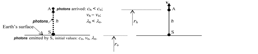
Referring to Harvard tower experiment [1] -[3] , simply represented on Figure 4, where h is the tower height, calling c0 the value of c on Earth’s surface at the tower base and ch its value on its top, the variation ch ‒ co) from the tower base to its top, from (11), for c = u, becomes
 (40)
(40)
where
 is the variation of the total gravitational potential U, due to Earth, from the
tower base to its top. As
is the variation of the total gravitational potential U, due to Earth, from the
tower base to its top. As
 and
and
 where ME is the Earth’s mass and r its radius, we get
 = MEGh/r2 where h (=rh ‒ ro) is
the tower height, yielding
= MEGh/r2 where h (=rh ‒ ro) is
the tower height, yielding
 (41)
(41)
showing that, on the top, where |Uh| < |Uo|, it is ch
< co, with .
.
 (a) (b)
Figure 4. Harvard tower experiment scheme, with the source at the base. (a) S and A at rest at a different level h. In A, λh < λo, so the detector observes a gravitational blue-shift; (b) Source and absorber relative motion (v) to compensate the gravitational blue-shift through the Doppler effect.
Now, let S be a Mossbauer source and A an appropriate absorber; if they are close to each other (for instance, at the tower base), the absorber is in resonance with the source.
Then, see Figure 4(a), with S at the tower base and taking A to its top, while S and A are at rest, the frequency of the emitted photons (i.e. the number of photons emitted along the direction SA per unit of time) has to be equal to the photons received by A, that is nh = no and since ch < co, it must be λh < λo (indeed Δλ/λo = Δc/co), so, contrary to ToR, a blue-shift effect for A.
[On Figure 4(a) (photons arrived to the top), according to nh = no, it seems to be Eh/Eo = hnh/hno = 1 (here h is the Planck constant), but the (33) shows that h = γc2 with γ (representing the mass of light passing during T along one ray), an effective constant, so that we get Eh/Eo = (ch/co)2 which shows a decrease of the energy of light from S to A].
Indeed, with S on the base emitting toward A on top, A goes out of resonance and since on our bases nh = no, the non-resonances physically related to a variation of λ, whereas in the Harvard tower experiment [3] , “no mention has been made of frequency or wavelength”.
Thus, to restore the resonance through the Doppler effect (i.e. to increase the photon length fromits value λh in A to its initial value λo in S), since λh < λo, A and S, see Figure 4(b), have to recede from each other with speed v complying with (17), here written λo = λh + vT, giving (λh ‒ λo)/λo = ‒vT/λo.
Therefore, since Δλ/λo = Δc/co (as no = nh),
we find Δc/co = ‒vT/λo and comparing to (41) we get , so the relative speed between S and A becomes
 (42)
(42)
[This value is also predicted by General Relativity (GR)which, implying a decrease of v for light moving from the base to the top, predicts an opposite direction of v with respect to the one shown on Figure 4(b); at this regard, Pound-Rebka [3] operated in order to determine (through the value of v, obtained moving the source sinusoidally) the variation of energy of a beam on the upward and downward path, without any indication (because of the low value of v), about the direction of the compensating speed].
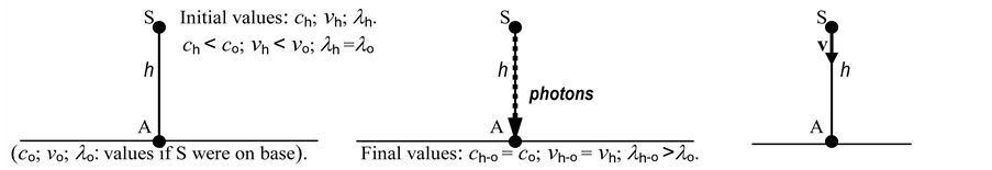
Now, if we take S to the tower top, with A located on its base (see Figure 5 which is referred on our bases), the experiment shows that the absorber goes out of resonance.
Now, according to Relativity, taking S to the top, the initial frequency of the
light should be nh = no, which, on our bases, is wrong: with
S on the top, see Figure 5(a), the (10) written
as c2 + 2U = 0, between top and base gives , where Uh ‒ U0
= gh, giving
, where Uh ‒ U0
= gh, giving , then
 , and since 2gh
= c2 we can write co = ch(1 + gh/c2), that is ch < co as showed by (41), but what about nh and λh?
Well, referring to previous Figure 4(a), with source
S on the base, the length of photons arriving to the to pvaries from λo
to λh (with λh < λo), therefore if S has been taken
now to the top, should their initial length be λh, at their arrival to
the base, their length should be λo, and since the resonance, as seen,
depends on λ, the Absorber A (on the base, see Figure 5(a)),
should be now in resonance. Thus we can argue that taking the source on top, the
photons initial length has to be λh (=λo); then, as ch
< co as shown by (41), it must be nh < no,
and in particu lar, according to (41) we get , giving
 which is the same as the one predicted by GR, but on our bases, this variation is
due to a different initial frequency (as the source is now on the top), whereas
for GR this variation is related to the path of the emitted light between two different
levels. (Indeed on our bases the frequency remains constant during any path, should
source and observer be at recipro-
which is the same as the one predicted by GR, but on our bases, this variation is
due to a different initial frequency (as the source is now on the top), whereas
for GR this variation is related to the path of the emitted light between two different
levels. (Indeed on our bases the frequency remains constant during any path, should
source and observer be at recipro-
 (a) (b) (c)
Figure 5. Harvard tower experiment scheme, with the source on the top. (a) S on top, S and A at rest: ch, nh, λh are the photons initial parameters on the tower top; (b) S and A at rest. When photons reach the base, λh-o > λo, so A observes a g-redshift; (c) S and A relative motion to compensate the g-redshift via Doppler effect.
cal rest).
Thus, see Figure 5(b), with S emitting from the top, S and A at rest, when the photons reach the base, as their final frequency (nh-0) will remain the same as the initial one (that is nh-o = nh) and since co > ch, it turns out that, along the path SA, λ will increase, and its variation, opposite to the one given by (41), yields now
 , giving
 .
.
Now, as λh-o > λo, the absorber, on the base, will observe a gravitational red-shift so, to compensate it via Doppler shift, see Figure 5(c), S and A have now to move relative to each other in order to decrease the final length λh-o to the resonance value λo; on the contrary, according to ToR, A and S should recede from each other.
[Still referring to Figure 5, taking S to the tower
top, we have ch < co and nh < no implying,
contrary to GR, a decrease of the energy of light to be emitted by S,
 , see (34), and therefore when these photons reach
the base (where ch-o = co) their energy becomes
, see (34), and therefore when these photons reach
the base (where ch-o = co) their energy becomes
 giving a reason to the loss of energy as for light arriving to Earth coming from
sources located in points where |US| < |Uo|, and since, as
seen,
giving a reason to the loss of energy as for light arriving to Earth coming from
sources located in points where |US| < |Uo|, and since, as
seen,
 , we also give a cosmological reason to the high
redshift of sources where |US| = |Uo|.
, we also give a cosmological reason to the high
redshift of sources where |US| = |Uo|.
Time Dilation
Well, the experience shows that, on board of GPS satellites, the atomic clocks run faster by about 38 μs/day than the ones on ground, meaning that, in altitude, their ticking time, (or interval time, intending the minimum time counted), is shorter than the one on ground.
Now, the ticking time t of atomic clocks is proportional to their frequency, so on ground we can write t0 = kv0 while in altitude th = knh yielding Δn/no = Δt/to where Δt (=th ‒ to) is the ticking time variation from ground to height h, with Δn (=nh ‒ no) representing their frequency variation due to the gravitational potential variation.
Now, taking the sources (clocks) from ground to height h, the length of their photons, at emission, remains constant, (λh = λo), thus, because of the variation of c (from ground to height h), it has to correspond an equal variation of n, so that the (40) can be written as
 (43)
(43)
Now, GPS satellites have an orbit of rh 26,600 km, that is an altitude h 20,200 km, as ro 6400 km is the Earth’s radius. Hence, the (43), because of the variation of the potential, the variation of the counted time during one day (Δt1d), since in one day t1d = 86,400 s, gives
 (44)
(44)
where the sign means that the ticking time is decreasing, inducing the clocks to run faster. Then we have to take into account that the parameters of the photons emitted by atomic clocks on board of GPS satellites are changing because they are circling around the Earth.
Therefore, according to (29), that is T' = T(1 + β2)1/2 where T' is the time a photon needs to cross the Observer, during one day (86,400 s), since the orbital speed corresponds to two orbits every day (giving v = 2(2πrh/86,400) = 3870 m×s-1, and considering that for v = c we can write (1 + β2)1/2 @ 1 +β2/2, we get
 (45)
(45)
representing the variation of the counted time in one day due to the orbital speed of GPS satellite, and since this variation is positive, it has to be deducted from the negative one due to the potential variation, thus the total variation of the counted time on GPS satellites, in one day, becomes
 (46)
(46)
as observed. This equality also confirms that λh = λo as for sources in altitude.
7. Red Shift
According to the Relativity, the gravitational red shift of light coming from the
Sun, with MS and RS its mass and radius, is . Now, for
 Mpc, with s the distance Earth-source, the observed shifts are in the range
 [12] , while from
 to
to
 Mpc they tend to become always positive, and between
 and
and
 Mpc (
Mpc ( Bly) the red shifts (here in the range
 ), practically follow the empirical
Hubble’s law z = Hos/c; hence, since the value of the gravitational red
shifts of a typical galaxy, intended to be
), practically follow the empirical
Hubble’s law z = Hos/c; hence, since the value of the gravitational red
shifts of a typical galaxy, intended to be
 should be of the order of 10-9, the Doppler effect appears
to be (as for the Relativity), the only satisfactory way to explain the observed
blue shifts and also the high (cosmological) red shifts.
should be of the order of 10-9, the Doppler effect appears
to be (as for the Relativity), the only satisfactory way to explain the observed
blue shifts and also the high (cosmological) red shifts.
On the contrary, on our basis, disregarding any motion between a source and an Observer
on Earth, which implies (as showed on §4) n = no, we get , where no,
co and λo are observed on Earth, showing that for co
> c, it has to be λo > λ. Hence, the blue/red shifts observed on Earth
can be expressed as
, where no,
co and λo are observed on Earth, showing that for co
> c, it has to be λo > λ. Hence, the blue/red shifts observed on Earth
can be expressed as
 (47)
(47)
where
 is the potential on Earth, while Us the one on the source (at distance
s). Thus the shift of a far source, disregarding the motion source-Earth, turns
out to be the variation of c (as well as λ) during the path of light toward a different
potential; for instance, going from Earth to Sun, and considering that along this
path the main variation of potential (ΔU(s)) is due to the Sun only,
we can write US = Uo + ΔU(s) where
is the potential on Earth, while Us the one on the source (at distance
s). Thus the shift of a far source, disregarding the motion source-Earth, turns
out to be the variation of c (as well as λ) during the path of light toward a different
potential; for instance, going from Earth to Sun, and considering that along this
path the main variation of potential (ΔU(s)) is due to the Sun only,
we can write US = Uo + ΔU(s) where
 (48)
(48)
With d the distance Earth-Sun; so on the Sun,
 and then
 (49)
(49)
giving , while on the opposite
path, Sun to Earth, it is
, while on the opposite
path, Sun to Earth, it is , hence a blueshift (contrary to
a red shift of the same value predicted by the Relativity).
, hence a blueshift (contrary to
a red shift of the same value predicted by the Relativity).
As for
 Mpc, according to (47), if Us (potential on the source) is, in absolute
value, higher than the potential on Earth Uo, we get, on Earth, z < 0
(blue shift), and vice versa for |Us| < |Uo|, hence, apart
Doppler effects, these red/blue shifts indicate that the potential, from Earth to
the sources in this space, may increase or decrease (and since for
Mpc, according to (47), if Us (potential on the source) is, in absolute
value, higher than the potential on Earth Uo, we get, on Earth, z < 0
(blue shift), and vice versa for |Us| < |Uo|, hence, apart
Doppler effects, these red/blue shifts indicate that the potential, from Earth to
the sources in this space, may increase or decrease (and since for
 Mpc, z is positive, we may also argue that our galaxy is close to the middle of
the masses of universe); then, over this distance, it turns out that, on the related
sources, US is (in absolute value), always lower than Uo,
and also tending to zero for z → ∞.
Mpc, z is positive, we may also argue that our galaxy is close to the middle of
the masses of universe); then, over this distance, it turns out that, on the related
sources, US is (in absolute value), always lower than Uo,
and also tending to zero for z → ∞.
In the range
 (where z follows the Hubble’s law), the (47), written as
 (50)
(50)
for z = 1 gives
 yielding (through a simple artifice) to
 (valid for z = 1) (51)
which shows that, for z = 1, Us depends linearly on z; in particular, Table 1 shows that, in the said range

Table 1 . Calculated values of U and c related to the observed redshifts on Earth. The 4th column is referred to Equation (50); the 5th to (51); the 6th to (47).
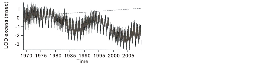
Figure 6. Length of day since 1969, when Earth-Moon laser ranging data started to be collected. The dotted line shows the 2.3 msec∙cy−1 trend expected as a consequence of momentum conservation, when it is assumed that, using laser ranging, an actual increase of Earth-Moon distance is measured. LOD data comes from the EOP 05. C04 series (Bizouard and Gambis 2009), as provided by the Earth Orientation Centre (http://hpiers.obspm.fr). The Figure has been taken from the paper of Sanejouand, Y.H., Empirical evidences in favour of avarying-speed-of-light, arXiv 0908.0249.
( ), the values given by (51), are practically the same as the
ones given by (50). Table 1 also shows the values
of U and c for various values of z.
), the values given by (51), are practically the same as the
ones given by (50). Table 1 also shows the values
of U and c for various values of z.
8. Conclusions
We showed that, on our basis, c corresponds to the total escape speed u which is practically constant on Earth (see §3), while the annual variations of c, due to the eccentricity of the Earth’s orbit, are well shown on following Figure 6.
In fact, when the Earth (on perihelion) approaches the Sun, because of the distortion of the shape of Earth, the angular speed of Earth should decrease, hence, the length of day (LOD)should increase; moreover, during the approach Earth-Sun, due to the increase of the absolute value (on Earth) of U, the speed of light (on Earth) has also to increase, thus the LOD and c should show, at the same time, annual peaks, as shown on Figure 1, which may also represent, in another scale, the annual variations of the speed of light, since 1969.
Now we point out our attention on Compton effect: indeed, through the relativistic Doppler effect equations, one cannot get the Compton equation (which can be found in other ways), whereas through our Doppler effect Equation (17), we can obtain it; well, one can observe that the Compton effect is not a Doppler effect, but in this case why we get the Compton equation? Is it a coincidence or the relativistic Doppler effect equations are not correct?
Finally, regarding the Harvard tower experiment, the Relativity, as for the compensating speed source-Observer (in order to restore the resonance between them), predicts opposite directions with respect to the ones we have obtained: we hope that now (after 50 years from the related experiment) an appropriate (similar) experiment will give a sure answer.
References
- Pound, R.V. and Rebka Jr., G.A. (1960) Physical Review Letters, 4, 337. http://dx.doi.org/10.1103/PhysRevLett.4.337
- Pound, R.V. and Snider, J.L. (1964) Physical Review Letters, 13, 539. http://dx.doi.org/10.1103/PhysRevLett.13.539
- Pound, R.V. and Snider, J.L. (1965) Physical Review, 140, B788. http://dx.doi.org/10.1103/PhysRev.140.B788
- Kragh, H. (1996) Cosmology and Controversy. Princeton University Press, Princeton, 212.
- Gogberashvili, M., et al. (2012) Cosmological Parameter. ArXiv:physics.gen-ph, 2.
- Immerman, N. (2001) Nat’l Solar Observatory: The Universe. University of Massachusetts, Sunspot.
- Gott III, J.R., et al. (2005) The Astrophysics Journal, 624, 463-484.
- Van Dokkum, P. (2010) Nature, 468, 940-942. http://dx.doi.org/10.1038/nature09578
- Schutz, B.F. (2003) Gravity from the Ground Up. Cambridge University Press, Cambridge, 361.http://dx.doi.org/10.1017/CBO9780511807800
- Halliday, D. and Resnic, R. (1981) Fundamental of Physics. John Wiley & Sons, New York.
- Mohr, P.J. and Taylor, B.N. (2000) Review of Modern Physics, 72, 351-495.
- (Yearly) NASA Extragalactic Database.
Appendix A (Compton Effect)
Here, see Figure A1, an incident photon (length
λ, frequency n), ejects a circling electron (me) but there is also a
reflected photon (length λ' frequency ) so the electron, while emitting
a photon λ' toward the Observer A, represents a source in motion from A along the
direction w, thus (considering the component wA of w) there is an indubitable
Doppler effect.
) so the electron, while emitting
a photon λ' toward the Observer A, represents a source in motion from A along the
direction w, thus (considering the component wA of w) there is an indubitable
Doppler effect.
Now, on the basis that the scattered photon starts to be reflected at the same time
when the incident photon starts to hit the electron, and since
 (=1/
(=1/ ) is the emission time of the
photon
) is the emission time of the
photon , it turns out that
 is also the whole interaction time, meaning that there is not a complete absorption
of the incident photon followed by an emission: this means that the internal energy
of the photon is not involved in this action, hence the momentum transferred from
the incident light to the electron is p = mc (=γc/T) as per (38), and the same value
p = mc is the momentum transferred from the scattered photon to the electron.
is also the whole interaction time, meaning that there is not a complete absorption
of the incident photon followed by an emission: this means that the internal energy
of the photon is not involved in this action, hence the momentum transferred from
the incident light to the electron is p = mc (=γc/T) as per (38), and the same value
p = mc is the momentum transferred from the scattered photon to the electron.
Therefore, the Conservation of Momentum (CoM) along the direction normal to w, becomes
 giving
 .
.
Moreover, the length of the reflected photon, for the Observer, according to (17) is
 (52)
(52)
where
 and where
 is the component of the electron speed along the direction of the Observer A and
 (=1/
(=1/ ) is, for A, the photon transit time, so we get
 (53)
(53)
Now the CoM along w is
 giving
 (54)
(54)
and plugging this value into (53) we get
 (55)
(55)
Now,
 , hence
 and therefore
 (56)
(56)
and since , we get the Compton equation:
 (57)
(57)
which cannot be obtained through the relativistic Doppler effect equation which,
as for a source receding from the Observer, is

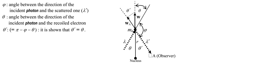
Figure A1. Compton effect.
Appendix B
Regarding the Conservation of Energy (CoE), E = U + K = 0, leading to
 the term K is the unitary (per unit of mass) kinetic energy of a massive particle,
hence as for the light (having total energy, see (34),
the term K is the unitary (per unit of mass) kinetic energy of a massive particle,
hence as for the light (having total energy, see (34),
 with Ki its internal energy), we
have to consider, to comply the CoE, its kinetic energy only, giving
with Ki its internal energy), we
have to consider, to comply the CoE, its kinetic energy only, giving , like any other
massive particle. Anyhow, one can observe that the internal energy of light (
, like any other
massive particle. Anyhow, one can observe that the internal energy of light ( ) of photons going toward the infinity could
be lost, but this is not the case: indeed, we have seen on §6 (see also Figure 4(a))
that the frequency of a photon is constant along its path, and since, see (34),
) of photons going toward the infinity could
be lost, but this is not the case: indeed, we have seen on §6 (see also Figure 4(a))
that the frequency of a photon is constant along its path, and since, see (34),
 , it turns out that toward the infinity, where
c∞ → 0, we get
, it turns out that toward the infinity, where
c∞ → 0, we get , yielding Ki∞
→ 0 (In other words, the internal energy of light only depends on the length of
their photons).
, yielding Ki∞
→ 0 (In other words, the internal energy of light only depends on the length of
their photons).