Applied Mathematics
Vol.08 No.07(2017), Article ID:78016,15 pages
10.4236/am.2017.87079
Construct Validation by Hierarchical Bayesian Concept Maps: An Application to the Transaction Cost Economics Theory of the Firm
Matilde Trevisani
Department of Economics, Business, Mathematics and Statistics “Bruno de Finetti”, University of Trieste, Trieste, Italy

Copyright © 2017 by author and Scientific Research Publishing Inc.
This work is licensed under the Creative Commons Attribution International License (CC BY 4.0).
http://creativecommons.org/licenses/by/4.0/


Received: June 29, 2017; Accepted: July 25, 2017; Published: July 28, 2017
ABSTRACT
A concept map is a diagram depicting relationships among concepts which is used as a knowledge representation tool in many knowledge domains. In this paper, we build on the modeling framework of Hui et al. (2008) in order to develop a concept map suitable for testing the empirical evidence of theories. We identify a theory by a set of core tenets each asserting that one set of independent variables affects one dependent variable, moreover every variable can have several operational definitions. Data consist of a selected sample of scientific articles from the empirical literature on the theory under investigation. Our “tenet map” features a number of complexities more than the original version. First the links are two-layer: first-layer links connect variables which are related in the test of the theory at issue; second-layer links represent connections which are found statistically significant. Besides, either layer matrix of link-formation probabilities is block-symmetric. In addition to a form of censoring which resembles the Hui et al. pruning step, observed maps are subject to a further censoring related to second-layer links. Still, we perform a full Bayesian analysis instead of adopting the empirical Bayes approach. Lastly, we develop a three-stage model which accounts for dependence either of data or of parameters. The investigation of the empirical support and consensus degree of new economic theories of the firm motivated the proposed methodology. In this paper, the Transaction Cost Economics view is tested by a tenet map analysis. Both the two-stage and the multilevel models identify the same tenets as the most corroborated by empirical evidence though the latter provides a more comprehensive and complex insight of relationships between constructs.
Keywords:
Concept Map, Graph Model, Hierarchical Bayesian Approach

1. Introduction
In its original form, a concept map is a graph model comprised of concepts and relationships between concepts. Concepts or nodes are usually enclosed in cir- cles or boxes of some type, relationships or links are indicated by a connecting line and a possible linking word between two concepts. It has been widely used in psychology, education, and more recently introduced in marketing [1] , knowledge management and intelligence [2] , as a means to understand indivi- dual mental representation of concept associations, and further, to understand how cognitive representations influence people’s subsequent behaviors and atti- tudes. Until the recent proposal of [3] , concept maps have been analysed heuris- tically or algorithmically by extracting and then using for analysis a set of sum- mary statistics. Hui et al. develop a probability model for concept maps that provides a unified modeling framework allowing for quantification of variation (e.g. by hypothesis testing) and proper summarization of information across individuals (e.g. by a consensus map construction). In particular, they extend the uniform graph model in two directions, by i) allowing for non-uniform pro- babilities of link-formation and by ii) introducing a latent pruning step to ensure that the generated maps are fully connected.
In this paper, we extend the modeling framework of Hui et al. in order to make it suitable for testing the empirical evidence of theories or main tenets of these. That is, we identify a theory by a set of core propositions, each, essentially asserting that one set of independent variables affects one dependent variable (besides main effects, interaction effects are considered as well). Moreover, every independent/dependent variable can have several operational definitions. Then, we propose an adapted version of concept map, that we call tenet map, to the context of theory testing. Here, data consist of a selected sample of scientific articles from the empirical literature on the theory under investigation and each article can include one or more (statistically rigorous) tests of the theory being assessed. Moreover, the overall independent and dependent variables as well as all the operational definitions of the variables comprise the potential nodes of any single map. Differently from Hui et al., links of a tenet map are two-layer: first-layer links show which connections between variables have been considered in the test at issue, second-layer links show which of them have been found statistically significant (in a direction consistent with the propositions of the theory) therein. In addition, the matrix of link-formation probabilities is, within either layer, block-symmetric (thus replacing the full-symmetric matrix in Hui et al.) since nodes are block-wise connected (not all the independent variables are connectable to every dependent variable and each variable is associated with a specific set of operational definitions). First layer probabilities describe the extent to which theory tenets have been acknowledged and applied in scientific research, second layer probabilities identify which of them have been more validated.
Similarly to Hui et al., observed maps are censored, i.e. a portion of complete (or potential) maps is missing. One form of censoring resembles the pruning step which Hui et al. have already accounted for: whether a construct node is missing, any associated link to measurement nodes is missing as well. But, in addition, tenet maps feature another form of censoring, this one similar to that arising in observational studies: whenever a first-layer link is missing the associated second-layer link is necessarily missing. In “concept mapping”, these censoring forms would be recognized, the first, as missingness of any higher- order link being missing any parent lower-order link, and, the second, as impos- sibility of labelling a link being it missing.
Finally, we perform a full Bayesian analysis instead of adopting the empirical Bayes approach followed by Hui et al. Actually, our model-based tenet map features some more complexities which have not been addressed in the original version. In addition to the complexities inherent to the connection structure above outlined (second-layer links and the further form of censoring associated with it), we show that the probabilistic structure can be furtherly enriched by developing a three-stage model which accounts for dependence either between data or within sets of parameters.
The case-example which motivated the development of tenet maps was the investigation of the empirical support and the degree of paradigm consensus of two leading theories of firm: the Transaction Cost Economics (TCE) and the Resource-Based View. Whether these two approaches can be considered as proper theories in alternative to the neoclassical paradigm of firm, is still de- bated. Purpose of the study is showing how a tenet map analysis can: a) help clarifying which and how many tenets (as well as the way they are practically operationalized) of a theory are more corroborated by empirical evidence by means of a consensus map which properly summarizes a set of individual maps; b) gauge the comparative success of one theory versus the other by comparing the correspondent consensus maps generated with different values for the strength of link probability. The remainder of the paper is organized as follows. In Section 2 we develop our statistical model of tenet maps. Section 3 describes the case-example and data, addressing in this paper the sole TCE theory. Finally, Section 4 presents some findings from the application of our model to data and concludes with directions for future research.
2. Model
2.1. Notations and Definitions
A theory is defined as a set of core propositions or tenets ( , ) each essentially consisting in a hypothesized relationship between one set of expla- natory variables and one response variable. Moreover, every response/explana- tory variable (or construct) can have several operational definitions (or mea- surements). We will use , , and to index, respectively, response variables ( ), explanatory variables ( ) and, in the order, their operational variables ( and ), whereas l or m will be utilized for denoting either type of variable ( with ). Each tenet corresponds to a definite set of pairs―and “definition sets” of individual tenets can be overlapping―but, in the current version of the proposed model, this further assignment of hypotheses to tenets can be overlooked.
Data are given by a selected―according to a set of established criteria―sam- ple of scientific articles from the empirical literature on the theory under in- vestigation. Each article can include one or more (statistically rigorous) tests ( , , with indexing the scientific articles) of the theory being assessed, whence, in total, we have tests for assessing the em- pirical evidence of the theory on focus. We will use i to denote one test―the basic data unit―regardless of the article to which it belongs.
Figure 1 presents an example of a tenet map which describes a particular test of the economic theory we will introduce later on. Likewise Hui et al., we define as an indicator that equals 1 if variable l appears in the tenet map associated with the i-th test, 0 otherwise. (When we need to refer to a defined type of variable, the generic will be accordingly changed into , , and , respectively denoting the corresponding indicators for response, explanatory and relative measurement variables.) Still, similarly to Hui et al., we define as an indicator that equals 1 if there is a link between variable l and m in the i-th tenet map, but, in addition, we define as an indicator that equals 1 if the relationship between the linked variables has been assessed as statistically significative. Significativity is depicted by bold links. Either indicator is otherwise set to 0.
2.2. Complete-Data and Observed-Data Likelihood
We are interested in assessing the extent to which the target tenets have been acknowledged and applied in empirical literature, and we assume to gauge it by the frequency of occurrence, in scientific articles, of tests associated with such tenets. Moreover, we wish to know which operational variables are mainly used to measure the constructs under comparison. Furthermore, we are interested in the frequency of significative tests for every tenet hypothesis.

Figure 1. Example of a tenet map.
Thus, let indicate the probability of occurrence of testing an hypothezed relationship between a response variable k and an explanatory variable h (within, in general, a multivariable test such as a multiple regression analysis). Likewise, (or ) denote the probability of occurrence of the construct k (or h) being measured by the operational variable p (or q)1. Besides, let indicate the probability of significative test on the hypothesized relationship being operationalized by pair. Likewise, will indirectly―i.e., through some form of operationalization, ―measure the probability of signifi- cative test on the hypothesized relationship between constructs k and h. In addition of main effects , interaction effects will be considered as well whenever they are hypothesized by the theory. Notation for probability of significative test relative to interaction effects is derived as above.
Observed data for each map, , consist of indicators identifying which relationships are subject to verification in test i ( and, in case interaction-links are present, ) as well as how they are operationalized ( , , in case, ) and whether they turn to be significative ( , in case, ). We note that in order to estimate the indirect measure of the probability of significative test on the hypothesized relationship between constructs k and h, , we will use the statistic that equals 1 if there is at least one , 0 otherwise.
1Hereinafter, for clarity of exposition, we specifically use index-pairs for identifying any “construct link” between a response variable k and an explanatory one h, and use for identifying “operational links”. According to a more general terminology, and identify first-order and second-order links respectively. Besides, indexes and , specifically connected to k and h constructs, will be used only when the context needs such a specification, otherwise they will be generically denoted as p and q.
Considering that object of our analysis is estimating the set of probability values as described above, observed data obviously do not provide the complete data from which a plain inference would otherwise be made. For instance, if a certain response or explanatory variable does not appear in one map (i.e. or equals 0 for some k or h), any operational variable measuring the missing construct cannot be observed either. Still, if one relationship hypothesis has not been contemplated in one test (i.e. for some pair), no information about its significativity can be drawn either. The first case is essentially a form of censoring (that resembles the pruning step of [3] ) whereas the second instance is a form of intentional missingness similar to the situation of unobserved potential outcomes under treatments not applied in an experiment [4] .
Thus, let denote the complete data consisting of indicators that could potentially be observed if every construct were operationalized as well as if every relationship were tested regardless of (or once pinpointed) the test actually carried out in the considered article. Besides, let denote the inclusion vector consisting of indicators for the observation of : if is observed, otherwise ; likewise works.
In the sequel densities will be generically denoted by square brackets so that joint, conditional and marginal forms appear, respectively, as , and with generic random variables. The usual marginalization by integration procedure will be denoted by forms such as . Now, let , , and indicate the collections of, respectively, potential data, observed data, inclusion indicators and parameters of interest across the generic index pair . Then, the complete-data likelihood as expressed by the joint density of complete data and inclusion vector given the parameters , is
#Math_86# (1)
Inclusion indicators not only depend on observed data ’s (expressed by ’s in (1)) but are deterministically determined by these, as their densities
(2)
clearly show. Thus complete-data likelihood (1) can be conveniently written as
(3)
in order to obtain the joint density of observed data and inclusion vector given parameters , that is what we call the observed-data likelihood. In fact this is correctly obtained by integrating out missing data from the complete-data likelihood as follows,
(4)
(5)
(6)
After straightforward calculations (5-6), observed-data likelihood is reduced to where observed data are jointly associated with 1-valued inclusion indicators solely (see (4)). Hereinafter, we will indicate simply as given that they are the same ( from (2)).
2.3. Hierarchical Bayesian Specification
We build a HB model for tenet maps and adopt a fully Bayesian viewpoint.
The most basic (full) HB model has a three-part structure. Let write it down in terms of the joint distribution of the variables involved in our particular application, that is observed data , focused parameters plus addi- tional model unknowns ,
(7)
The first term on the right side of (7) is the observed-data likelihood which, under the above assumptions (taking to (6)), has the following form
(8)
The second term of (7) is the conditional prior of first-stage parameters. In the simplest version of our model, independence is assumed throughout the parameters. Besides, a natural prior for modeling frequency variables is the beta distribution. Thereby,
(9)
(10)
(with ) so that, at prior, , , and for every index pair . The parameterization adopted for Beta ( , and analogously for ) has been chosen because of its direct interpretation and convenience when modeling hyperprior distribution. In fact, we are now at the third term on the right side of (7), the prior distribution of hyperparameters or the parameters set at the basis of the hierarchical structure. Because we have no immediately available information about the distribution of q’s and l’s, we use a noninfor- mative hyperprior distribution. In particular, we assign independent uniform priors over the range ,
(11)
Alternatively, one can put independent reference (or Jeffrey’s) priors, i.e.
(12)
(the same for ) or a mixed composition of (11) and (12), i.e. (either order). Each one choice is a proper prior, thus ensuring a proper posterior, but reflects different attitudes towards the idea of non-informativeness [13] . A sensitivity analysis will be carried out by using them all.
HB way of thinking easily allows to make model adequately complex, so as to make it better suited to cope with the problem under investigation. We mention two possible extensions of the basic two-stage model (7). First, we can relax the independence assumption set throughout the frequency parameters. For instance, each set of parameters associated with an hypothesized rela- tionship between a given set of explanatory variables and one response variable k, is likely to be positively correlated. In such a case, dependence can be properly introduced by adding a further level to the hierarchy (7) that describes the distribution of across multivariate tests associated with one response variable k. In detail, in (9) can be furtherly decomposed into two com- ponents
(13)
where operational link parameters, and , are modeled as before, whereas each set , with k fixed, shares an individualized hyperparameter . Again, a beta prior can be assigned to each with parameters , i.e. in (13), as well as to every frequency mean , i.e. , with parameters here set equal to the founder hyperparameters of process. A similar prior hierarchy (beta- beta) has proved to be an effective strategy in other application fields (e.g. for modeling allele frequency correlations in a geographical genetics study; see Chapter 2 of [5] in this regard). As usual, a flat prior can be given to the scale parameter .
As a consequence of (13), any pair of parameters are, conditional to and , marginally correlated. Their covariance in fact is , whilst is null for any pair with different k. Besides, and , whence . Correlation tends to 1 if approxi- mates zero whereas tends to its minimum value, , if approximates 1: closer the to zero, smaller the variance of (and more similar the ’s are) across k’s, viceversa for tending to 1.
Second, we can make model (7) more flexible by adding a further level which accounts for the nested structure of tests within articles (recall we have test , , within article ). Again, we can furtherly decompose in (9) so that the basic specification (7) becomes a three-stage model as follows,
(14)
More in detail, likelihood (8) here changes only in that part depending on , that is
(15)
to stress that tests within the same article usually verify relationships between a definite set of constructs and use a definite set of operational measures, whereas the significance of tests is not necessarily correlated. Besides, article level para- meters, , are modeled as Beta’s centered on this way
(16)
Differently from the first extension, (13), which was introduced to model possible dependencies between parameters, the multilevel specification, (14), addresses the problem of properly weighting first-level data (single tests) for inference on relevant parameters. That is, it aggregates test-level data to inform on article-level parameters, , which in turn inform on global parameters .
For inference, we used MCMC methods and implemented a Gibbs sampler. Full conditionals for (of models (7) and (13)), (of model (14)), and parameters are beta distributions (beta prior being conjugate with a binomial likelihood). Whilst, full conditionals for parameters (of model (14)) and hyperparameters , (of model extensions), and have not a closed form. A slice sampler (within Gibbs) has been then worked out (which proved to be more efficient than a Metropolis step).
3. Application
3.1. TCE: A New Theory of the Firm
There is a widespread opinion that, still nowadays, economic theory has not yet developed a complete theory of the firm. The dominant paradigm is the neo- classical one which identifies the firm as a production function transforming inputs in outputs. But, the production process is critically said to be treated like a black box. In these last decades, two alternative approaches―which try to open the black box―have mainly emerged: the Transaction Cost Economics (TCE) and the Resource-Based View. Yet debate continues regarding their empirical support and degree of consensus.
With regard to the TCE, we consider the central tenets as originally elaborated by Williamson [6] [7] [8] [9] [10] , though there exist anticipating ideas and some elaborations and extensions of the theory. The TCE describes firms as governance structures and, focusing on transactions (transfers of good or ser- vice), claims that the choice of governance mode is directed towards minimizing transaction costs. Factors like bounded rationality and opportunism are the underlying conditions assumed by the theory to explain the existence of trans- action costs. The central hypothesis is what is called the “discriminating align- ment hypothesis” according to which “transactions, which differ in their attributes, are aligned with governance structures, which differ in their cost and competence, so as to effect a transaction cost economizing result”. The principal attributes of transactions are asset specificity, uncertainty, and frequency, whereas the alternate forms of transaction governance identified by the theory are market, hybrid and hierarchy.
In synthesis, the propositions commonly regarded as the core tenets of the TCE [11] [12] for which we set out to gauge the level of empirical support are:
1) As asset specificity increases, hybrid and hierarchy become preferred over market; at high levels of asset specificity, hierarchy becomes the preferred governance form.
2) When asset specificity is present to a nontrivial degree, increases in uncer- tainty increase the relative attractiveness of hierarchies and hybrids.
3) When asset specificity is present to a nontrivial degree, high uncertainty renders markets preferable to hybrids, and hierarchies preferable to both hybrids and markets.
4) When both asset specificity and uncertainty are high, hierarchy is the most cost-effective governance mode.
5) Hierarchy will be relatively more efficient with recurrent transactions, and when either asset specificity is high and uncertainty is either high or medium, or when asset specificity is medium and uncertainty is high.
6) Trilateral governance (a hybrid relationship) will be efficient for transac- tions that are occasional, have intermediate levels of uncertainty and have either high or medium asset specificity; bilateral governance (a hybrid relationship) will be efficient for transactions that are recurrent, have intermediate levels of uncertainty, and medium asset specificity.
7) Governance modes that are aligned with transaction characteristics should display performance advantages over other modes.
Chart 1 graphically displays the first six tenets listed above: right-most column shows the governance mode (green = market, orchid = hybrid, orange = hierarchy) as should be aligned with levels (l = low, m = medium, h = high) of specificity (tenet 1); the rest of the columns show governance mode for each relevant combination of attribute levels according to the correspondent tenet (from 2 to 6).
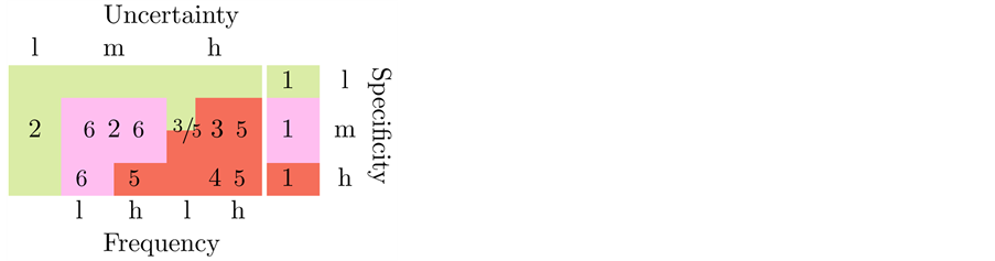
Chart 1. Core tenets of TCE: influence of transaction charac- teristics on governance mode.
3.2. Empirical Operationalization
The majority of empirical research in TCE is a variation of the discriminating alignment hypothesis mentioned above. In general, governance mode is the dependent variable, while transactional properties, as well as other related or control variables, serve as independent variables.
To assess the empirical evidence for the TCE, we analyzed 47 articles, selected according to a set of established criteria (see [11] [12] as reference works), with 130 tests of the theory and 650 statistical (1-predictor) tests in total. Chart 2 displays the overall constructs by which the dependent and independent variables have been conceptualized. Constructs acting as dependent variable are broadly of three types: organizational form ( with k from 1 to 6), perfor- mance of governance form (from 7 to 9), and the level of transaction costs (10,11). Coded independent variables are of four types: transaction characteris- tics that raise transaction costs ( with h from 1 to 13), transaction costs (14, 15), governance forms (16) and control variables (17). Besides, also the inter- actions of asset specificity and uncertainty categories―which comprise the only type of interaction effect found in the examined articles―have been included as constructs in the analysis.
Tenets possibly concerned with a combination of dependent and independent variables are indicated in the corresponding cell of the table (empty cells cor- respond to associations which are not explicitly taken into account by tenets).
With regard to the measures by which constructs have been operationalized, we have tried at best to combine a myriad of indicators into the smallest set of univocal concepts. Chart 3 shows how some of the dependent as well as inde- pendent variables have been practically measured in the studies under examina- tion. For instance, construct (hierarchy vs. market) can be operationalized as (in-house production vs. external purchase), (direct vs. represen- tative salespeople), etc.; (vertical integration) can be measured by (value added/sales), (number of supervisory levels), etc., and so on.
An example of a test of the TCE theory represented by a tenet map is illustrated in Figure 1. This particular test consists of a multiple regression of response va- riable (hierarchy vs. market)―measured by (direct vs. representative salespeople)―on explanatory variables (human assets), (market uncer-tainty), (behavioral uncertainty) and (control variable)―res-

Chart 2. Theoretical constructs: dependent and independent variables.
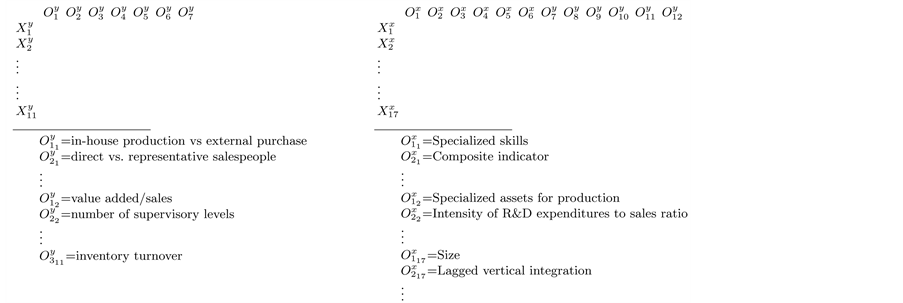
Chart 3. Operational constructs: dependent variable (left) and independent variables (right).
pectively measured by (composite indicator), (demand changes), (performance evaluation) and (size)―plus two interaction variables and . The only predictors which resulted significative (at 0.05 significativity level which was set throughout the tests from the selected set of articles) were , and . Thereby, this, say, i-th map provides us with data where with and , with equal to and , with , with equal to , where is and is , and where and are all 1-valued, the rest being throughout 0. The matricial coding of tenet maps utilizes a tabular representation like that of Chart 2 and Chart 3.
4. Model-Based Analysis of Tenet Maps
4.1. First Findings
We applied our proposed model set as in (7) and (14) versions to the data described above. Many are the outcomes of interest from the fit of a model- based tenet map. However, here we only mention someone and dwell on the most (statistically) attractive.
At link level, posterior estimates and intervals are immediately obtained for: (i) the probability of occurrence of any construct or operational link, i.e. for any and respectively; (ii) the probability of occurrence of finding a (statistically) significative relationship between any pair of constructs operationalized by a pair of measures, i.e. for any and indirectly for the relative .
On this regard, we mention that a sensitivity analysis was conducted by using the different hyperparameter priors before mentioned. Reference priors (12) lead to more extreme results than standard uniform priors: posterior intervals shift― as well as widen―towards 0 or 1. (That also affects the consensus map genera- tion which we describe below.)
At concept level, posterior estimates of construct “centrality” can be obtained by estimating row sums and , which roughly correspond to the occurrence of k dependent and, respectively, h independent constructs.
At map level, a “consensus map” can be easily constructed by: first, specifying a “cutoff” value c of probability of occurrence―thought to be large enough for assuring a certain degree of consensus; second, generating a latent map where and if the posterior estimates of the correspondent pro- babilities and are , 0 otherwise; lastly, obtaining the realized consensus map by “pruning” the latent map . This last step consists in deleting every operational link k-p or h-q wherever the theoretical construct k or h is not present on the map. Likewise, every significance link p-q as well as k-h is to be deleted if the correspondent underlying y-link is not present.
We generated the consensus map for the TCE by setting different values for c and compared the findings of the two-stage model (7) with those of the multilevel version (14). Figure 2 shows the results obtained with (an intermediate value). In synthesis, tenets 2 and related 3,4 are the most applied propositions in empirical studies; moreover, asset specificity proves to be the most validated attribute of the theory. Though a deeper interpretation of results is needed, it is beyond the objective of the paper. However, some differences result from fitting the two model versions. As we anticipated, multilevel model is informed by test-level data through aggregation on article- level. Thus, if there is less variability within articles than between them―as it is in our sample set―then the probability mass of the fitted two-stage model tends to be concentrated on fewer relationships or tenets than the correspondent multilevel version.
4.2. Conclusions and Future Directions
In this paper, we extend the modeling framework of Hui et al. in order to make concept mapping suitable for testing the empirical evidence of theories, in particular to gauge the extent to which main tenets of a theory have been acknowledged and applied in scientific research and to identify which of them
 (a)
(a)  (b)
(b)
Figure 2. Consensus map from two-stage model (a) and multilevel model (b).
have been more validated. Then we develop a model-based analysis of “tenet maps” consisting in a two-stage HB model―the basic form (7)―and a multilevel version (14). By our models we are able to obtain the degree of centrality for any construct of a theory and the mapping of paradigm consensus.
Concluding, several model developments can be envisioned. In particular, we are thinking of: modeling a possible dependence of parameters (that, we recall, measure the probability of a tenet hypothesis resulting in a significative test) on parameters (that measure the probability of a tenet hypothesis being tested), e.g. to explore how the significance of one predictor depends on the presence of other predictors in multiple regression; adding a further layer of parameters, , associated with tenet level j, to account for overlapping sets of tenet hypotheses; make random the cutoff values for consensus map cons- truction, e.g. generated by a Bayesian variable selection.
Cite this paper
Trevisani, M. (2017) Construct Validation by Hierarchi- cal Bayesian Concept Maps: An Application to the Transaction Cost Economics Theory of the Firm. Applied Mathematics, 8, 1016-1030. https://doi.org/10.4236/am.2017.87079
References
- 1. John, D.R., Loken, B., Kim, K. and Monga, A.B. (2008) Brand Concept Maps: A Methodology for Identifying Brand Association Networks. Journal of Marketing Research, 43, 549-563. https://doi.org/10.1509/jmkr.43.4.549
- 2. Medina, D., Martínez, N., Zenaida García, Z., del Carmen Chávez, M. and García Lorenzo, M.M. (2007) Putting Artificial Intelligence Techniques into a Concept Map to Build Educational Tools. In: Mira, J. and álvarez, J.R., Eds., Nature Inspired Problem-Solving Methods in Knowledge Engineering, Lecture Notes in Computer Science, Vol. 4528, Springer, Berlin, 617-627. https://doi.org/10.1007/978-3-540-73055-2_64
- 3. Hui, S.K., Huang, Y. and George, E.I. (2008) Model-Based Analysis of Concept Maps. Bayesian Analysis, 3, 479-512. https://doi.org/10.1214/08-BA319
- 4. Gelman, A., Carlin, J.B., Stern, H.S. and Rubin, D.B. (2004) Bayesian Data Analysis. 2nd Edition, Chapman & Hall/CRC.
- 5. Clark, J.S. and Gelfand, A.E. (2006) Hierarchical Modelling for the Environmental Sciences. Oxford University Press, New York.
- 6. Williamson, O.E. (1975) Markets and Hierarchies: Analysis and Antitrust Implications. Free Press, New York.
- 7. Williamson, O.E. (1981) The Economics of Organization: The Transaction Cost Approach. American Journal of Sociology, 87, 548-577. https://doi.org/10.1086/227496
- 8. Williamson, O.E. (1985) The Economic Institutions of Capitalism. Free Press, New York.
- 9. Williamson, O.E. (1991) Strategizing, Economizing, and Economic Organization. Strategic Management Journal, 12, 75-94. https://doi.org/10.1002/smj.4250121007
- 10. Williamson, O.E. (1991) Comparative Economic Organization: The Analysis of Discrete Structural Alternatives. Administrative Science Quarterly, 36, 269-296. https://doi.org/10.2307/2393356
- 11. David, R.J. and Han, S-K. (2004) A Systematic Assessment of the Empirical Support for Transaction Cost Economics. Strategic Management Journal, 25, 39-58. https://doi.org/10.1002/smj.359
- 12. Richman, B.D. and Macher, J. (2006) Transaction Cost Economics: An Assessment of Empirical Research in the Social Sciences. Duke Law School Legal Studies Paper, No. 115. http://ssrn.com/abstract=924192
- 13. Zhu, M. and Lu, A.Y. (2004) The Counter-Intuitive Non-Informative Prior for the Bernoulli Family. Journal of Statistics Education, 12, 1-10.