Received 1 April 2016; accepted 26 July 2016; published 29 July 2016

ABSTRACT

In this paper, we propose a new second order numerical scheme for solving backward stochastic differential equations with jumps with the generator linearly depending on. And we theoretically prove that the convergence rates of them are of second order for solving and of first order for solving and in norm.

Keywords:

Numerical Scheme, Error Estimates, Backward Stochastic Differential Equations

1. Introduction

Bismut (1973) studied the existence of the linear backward stochastic differential equation, the results could be regarded as a promotion of a famous Girsanov theorem. The existence and uniqueness of solutions for nonlinear backward stochastic differential equations (BSDEs) were first proved by Pardoux and Peng (1990).Since then, BSDEs have been extensively studied by many researchers. In [1] , Peng obtained the relation between the backward stochastic differntial equation and the parabolic partial differential equation (PDE), and in Peng (1990), the stochastic maximum principle for optimal control problems were based on BSDEs. The applications of BSDEs now cover many scientific fields, such as stochastic control, stock markets, risk measure, turbulence fluid flow, biology, chemical reactions, partial differential equations, and so on. Thus it is very important and useful to obtain solutions of BSDEs for real applications. However, it is often quite difficult to obtain analytic solutions of BSDEs, so computing approximate solutions of BSDEs become highly desired, by using the relation between the BSDE and PDE. As far as we know, there have been very few schemes obtained with second-order convergence rate, such as [2] [3] .

In this paper, we propose a new second order numerical scheme for the solution of forward-backward sto- chastic differential qquations (FBSDE in short) with jumps with the following form

(1)

From [4] , we know that the solution can be represented as

(2)

where the vector function is the classical solution of the following parabolic differential equation (PDE) of the form

(3)

where denotes the gradient of u with respect to the space variable x,

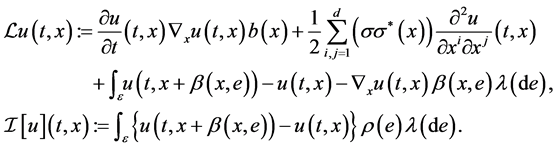(4)

2. Preliminaries and Notation

Let T be a fixed positive number and be a complete,filtered probability space on which is

defined a standard Brownian motion, such that is the natural filtration of the Brownian motion

and all the P-null sets are augmented to each s-field. Denote by the set of all -adapted and mean-square-integrable processes.

A process is called an -adapted solution of the FBSDE(1) if it’s -adapted and -integrable, and satisfies (1). Under some standard conditions on the functions f and h, there is a unique adapted random process.

Now we introduce a new probability space: for is an exponential martingale and satisfies

, we define. The random processes, it is easy to verify that is an exponential martingale.

(5)

Let us first introduce the following lemma.

Lemma 1. Given the time partition, X is a -measurable random variable,and satisfies.

(6)

We use the following Itô-Taylor approximation to solve the forward SDEs with jumps

(7)

where

(8)

and the coefficient function

(9)

with

(10)

Now we introduce some basic notations.

・ : the s-field generated by the Brownian motion.

・ Throughout this paper, we denote by C a generic constant depending only on T, the upper bounds of the derivatives of the functions f.

3. Numerical Schemes for Solving BSDE

From the time interval, we introduce the following time partition:, let

and. According to (1), it’s easy to obtain that for,

(11)

From (5) and (11),we have

(12)

(13)

(14)

From (12), (13) and (14), by applying Itô formula to, we obtain the equation

(15)

From (15), it is easy to obtain that for,

(16)

Taking the conditional mathematical expectation on both side of the obtained equation, and by the nature of the conditional mathematical expectation,we deduce

(17)

Based on (17), we have

(18)

where

(19)

and

(20)

According to Lemma 1, the equality, we have

(21)

Let for. Then is a standard Brownian motion with mean zero and vari- ance. Now multiply (11) by, taking the conditional mathematical expectation on both sides of the obtained equation, and using the Itô isometric formula, we deduce

(22)

From (22) we have,

(23)

where

(24)

Let, similarly multiplying (11) by yields

(25)

From (25) we have,

(26)

where

(27)

Based on (21), (23) and (26), for solving the BSDE (1) we propose the following scheme.

Scheme 1. Given, solve backwardly by

4. Error Estimates

In this section, we will give the error estimates of Scheme 1 proposed in Section 3. Now we introduce the error

, and in norm, where is the

solution of the FBSDEs (1), and is the solution of Scheme 1. For the sake of simplicity, we only consider one-dimensional BSDEs. However, all error estimate that we obtain in the sequel also hold for general multidimensional BSDEs. In our error analysis, we will use a constraint on the time partition step:

(32)

Let us introduce the following Lemma, its proof can be found in the reference [2] .

Lemma 2. Let, and () be the truncation errors defined in (21), (23) and (26), respec- tively. It holds that

(33)

(34)

Here C is a positive constant depending on T. We first give the error estimate for in the following theorem.

Theorem 1. Let () be the solution of the FBSDE (1) and

be the solution of Scheme 1. Assume. Then for sufficiently small time step, we have

(35)

for, where C is a constant depending on T.

Proof. Let. Subtracting (29) from (21) to get

(36)

Under the conditions of the theorem and by Lemma 2,we deduce that,

(37)

where L is the Lipschitz constant of with respect to y. Applying the inequality

for with,

, and, we deduce,

(38)

which by the inequality gives

(39)

Taking the mathematical expectation on both sides of (35), for sufficiently small we have

(40)

for. The terminal condition, the time step constraint (28) and the inequality

(41)

lead to for. The proof is completed.

Then we turn to estimating the error.

Theorem 2. Let be the solution of the FBSDE(1) and be the solution of Scheme 1. Assume. Then for sufficiently small time step, we have

for,where C is a constant depending on T.

Proof. Let. From (19) and (25), we get

By Lemma 2, the inequality and Hölder’s inequality, we deduce

(42)

where is a positive number which depends on p and the constant C in Lemma 2. Taking the mathematical expectation on both sides of the Equation (38) gives

(43)

by using Theorem 1 and constraint (28), leads to for. The proof is completed.

At last, we estimate the error.

Theorem 3. Let be the solution of the FBSDE(1) and be the solution of Scheme 1. Assume. Then for sufficiently small time step, we have

(44)

for, where C is a constant depending on T.

Proof. Let. From (26) and (31),we get

(45)

By Lemma 2, the inequality and Hölder’s inequality, we deduce

(46)

where is a positive number which depends on p and the constant C in Lemma 2. Taking the mathematical expectation on both sides of the Equation (42) gives

(47)

by using Theorem 1 and constraint (28), leads to for. The proof is completed.

Cite this paper

Hongqiang Zhou,Yang Li,Zhe Wang, (2016) A New Second Order Numerical Scheme for Solving Forward Backward Stochastic Differential Equations with Jumps. Applied Mathematics,07,1408-1414. doi: 10.4236/am.2016.712121

References

- 1. Pardoux, E. and Peng, S. (1990) Adapted Solution of a Backward Stochastic Differntial Equation. Systems & Control Letters, 14, 55-61.
http://dx.doi.org/10.1016/0167-6911(90)90082-6 - 2. Li, Y. and Zhao, W. (2010) Lp-Error Estimates for Numerical Schemes for Solving Certain Kinds of Backward Stochastic Differential Equations. Statistics and Probability Letters, 80, 21-22, 1612-1617.
- 3. Zhao, W., Chen, L. and Peng, S. (2006) A New Kind of Accurate Numerical Method for Backward Stochastic Differential Equations. SIAM Journal on Scientific Computing, 28, 1563-1581.
http://dx.doi.org/10.1137/05063341X - 4. Tang, S. and Li, X. (1994) Necessary Conditions for Optimal Control of Stochastic Systems with Random Jumps. SIAM Journal on Control and Optimization, 32, 1447-1475.
http://dx.doi.org/10.1137/S0363012992233858