Received 28 January 2016; accepted 26 February 2016; published 29 February 2016

ABSTRACT

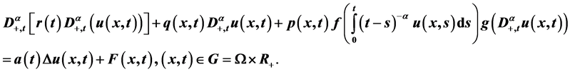
In this article, we will establish sufficient conditions for the interval oscillation of fractional partial differential equations of the form

It is based on the information only on a sequence of subintervals of the time space rather than whole half line. We consider f to be monotonous and non monotonous. By using a generalized Riccati technique, integral averaging method, Philos type kernals and new interval oscillation criteria are established. We also present some examples to illustrate our main results.

Keywords:

Fractional, Parabolic, Oscillation, Fractional Differential Equation, Damping

1. Introduction

Fractional differential equations are now recognized as an excellent source of knowledge in modelling dynamical processes in self similar and porous structures, electrical networks, probability and statistics, visco elasticity, electro chemistry of corrosion, electro dynamics of complex medium, polymer rheology, industrial robotics, economics, biotechnology, etc. For the theory and applications of fractional differential equations, we refer the monographs and journals in the literature [1] -[10] . The study of oscillation and other asymptotic properties of solutions of fractional order differential equations has attracted a good bit of attention in the past few years [11] -[13] . In the last few years, the fundamental theory of fractional partial differential equations with deviating arguments has undergone intensive development [14] -[22] . The qualitative theory of this class of equations is still in an initial stage of development.

In 1965, Wong and Burton [23] studied the differential equations of the form

In 1970, Burton and Grimer [24] has been investigated the qualitative properties of

In 2009, Nandakumaran and Panigrahi [25] derived the oscillatory behavior of nonlinear homogeneous differential equations of the form

Formulation of the Problems

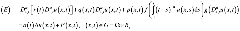
In this article, we wish to study the interval oscillatory behavior of non linear fractional partial differential equations with damping term of the form

where is a bounded domain in with a piecewise smooth boundary is a constant, is the Riemann-Liouville fractional derivative of order α of u with respect to t and ∆ is the Laplacian operator in

the Euclidean N-space (ie)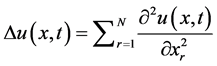. Equation (E) is supplemented with the Neumann

boundary condition

where γ denotes the unit exterior normal vector to and is a non negative continuous function on and

In what follows, we always assume without mentioning that

;

;, with on any for some

is convex with for.

is continuous where.

By a solution of, and we mean a non trivial function with

, and satisfies and the boundary conditions

and. A solution of, or, is said to be oscillatory in g if it has arbitrary large zeros; otherwise, it is nonoscillatory. An Equation is called oscillatory if all its solutions are oscillatory. To the best of our knowledge, nothing is known regarding the interval oscillation criteria of (E), (B₁) and (E), (B₂) upto now. Motivativated by [22] -[25] , we will establish new interval oscillation criteria for (E), (B₁) and (E), (B₂). Our results are essentially new.

Definition 1.1. A function belongs to a function class P denoted by if where which satisfies, for t > s and has partial derivatives

and on d such that

where.

2. Preliminaries

In this section, we will see the definitions of fractional derivatives and integrals. In this paper, we use the Riemann-Liouville left sided definition on the half axis. The following notations will be used for the convenience.

(1)

For denote

Definition 2.1 [2] The Riemann-Liouville fractional partial derivative of order with respect to t of a function is given by

provided the right hand side is pointwise defined on where is the gamma function.

Definition 2.2 [2] The Riemann-Liouville fractional integral of order of a function on the half-axis is given by

provided the right hand side is pointwise defined on.

Definition 2.3 [2] The Riemann-Liouville fractional derivative of order of a function on the half-axis is given by

provided the right hand side is pointwise defined on where is the ceiling function of α.

Lemma 2.1 Let y be solution of and

(2)

Then

(3)

3. Oscillation with Monotonicity of f(x) of (E) and (B₁)

In this section, we assume that f is monotonous and satisfies the condition where M is a constant.

Theorem 3.1 If the fractional differential inequality

(4)

has no eventually positive solution, then every solution of and is oscillatory in, where.

Proof. Suppose to the contrary that there is a non oscillatory solution of the problem (E) and which has no zero in for some Without loss of generality, we may assume that in,. Integrating (E) with respect to x over, we have

(5)

Using Green’s formula and boundary condition, it follows that

(6)

(7)

By Jensen’s inequality and we get

By using we have

(8)

In view of (1), (6)-(8), (5) yield

Take, therefore

Therefore is eventually positive solution of (4). This contradicts the hypothesis and completes the proof.

Remark 3.1 Let

Then we use this transformation in (4). The inequality becomes

(9)

Theorem (3.1) can be stated as, if the differential inequality

has no eventually positive solution then every solution of (E) and (B₁) is oscillatory in where.

Theorem 3.2 Suppose that the conditions (A₁) - (A₅) hold. Assume that for any there exist, , for such that, satisfying

(10)

If there exist, and such that

(11)

where and are defined as

Then every solution of, is oscillatory in G.

Proof. Suppose to the contrary that be a non oscillatory solution of the problem, say in for some. Define the following Riccati transformation function

Then for

By using and inequality (4) we get

(12)

By assumption, if then we can choose with such that on the interval. If then we can choose with such that on the interval So

therefore inequality (12) becomes

(13)

Let, , , , , ,.

Then, , , so (13) is transformed into

That is

(14)

Let be an arbitrary point in substituting with s multiplying both sides of (14) by

and integrating it over for we obtain

Letting and dividing both sides by

(15)

On the other hand, substituting by s multiply both sides of (14) by and integrating it over for we obtain

Letting and dividing both sides by

(16)

Now we claim that every non trivial solution of differential inequality (9) has atleast one zero in.

Suppose the contrary. By remark, without loss of generality, we may assume that there is a solution of (9) such that for. Adding (15) and (16) we get the inequality

which contradicts the assumption (11). Thus the claim holds.

We consider a sequence such that as. By the assumptions of the theorem for each there exist such that and (11) holds with replaced by respectively for . From that, every non trivial solution of (9) has

at least one zero in. Noting that we see that every solution has ar-

bitrary large zero. This contradicts the fact that is non oscillatory by (9) and the assumption in for some. Hence every solution of the problem, is oscillatory in G.

Theorem 3.3 Assume that the conditions (A₁) - (A₅) hold. Assume that there exist such that for any ,

(17)

and

(18)

where and are defined as in Theorem 3.2. Then every solution of is oscillatory in G.

Proof. For any, that is, , let,. In (17) take. Then there exists such that

(19)

In (18) take. Then there exist such that

(20)

Dividing Equations (19) and (20) by and respectively and adding we get

Then it follows by theorem 3.2 that every solution of is oscillatory in G.

Consider the special case then

Thus for we have and we note them by. The subclass containing such is denoted by. Applying Theorem 3.2 to we obtain the following result.

Theorem 3.4 Suppose that conditions (A₁) - (A₅) hold. If for each there exists and with such that

(21)

where and are defined as in Theorem 3.2. Then, every solution of and is oscillatory in G.

Proof. Let for that is then

For any we have

From (21) we have

since we have

Hence every solution of is oscillatory in G by Theorem 3.2.

Let where is a constant. Then, the sufficient conditions (17) and (18) can be modified in the form

(22)

(23)

Corollary 3.1 Assume that the conditions (A₁) - (A₅) hold. Assume for each i = 1, 2 that is and for some we have

and

.

Then every solution of and is oscillatory in G.

Theorem 3.5 Suppose that the conditions (A₁) - (A₅) hold. If for each i = 1, 2 and for some satisfies the following conditions

and

Then every solution of and is oscillatory in G.

Proof. Clearly,.

Note that

and

Consider

Similarly we can prove other inequality

Next we consider, where λ is a constant and and.

Theorem 3.6 Assume that the conditions (A₁) - (A₅) hold. If for each i = 1, 2 and for some such that

and

Then every solution of and is oscillatory in G.

Proof. From (17)

Similarly we can prove that

If we choose and we have the following corollaries.

Corollary 3.2 Suppose that the conditions (A₁) - (A₅) hold. Assume for each i = 1, 2 that is and for some we have

and

Then every solution of and is oscillatory in G.

Corollary 3.3 Suppose that the conditions (A₁) - (A₅) hold. Assume for each that and for some we have

and

Then every solution of and is oscillatory in G.

4. Oscillation without Monotonicity of f(x) of (E) and (B₁)

We now consider non monotonous situation

Theorem 4.1 Suppose that the conditions (A₁) - (A₄) and (A₆) hold. Assume that for any there exist, , for such that, satisfying

(24)

If there exist and such that

(25)

where and are defined as

Then every solution of, is oscillatory in G.

Proof. Suppose to the contrary that be a non oscillatory solution of the problem, say in for some. Define the Riccati transformation function

Then for

By using and inequality (4) we get

(26)

By assumption, if then we can choose with such that on the in-

terval. If then we can choose with such that On the in-

terval So

Therefore inequality (26) becomes

(27)

Let, , , , , ,.

Then, , , , so (27) is trans- formed into

where

that is

The remaining part of the proof is the same as that of theorem 3.2 in section 3, and hence omitted.

Corollary 4.1 Suppose that the conditions (A₁) - (A₄) and (A₆) hold. Assume for each that is and for some we have

and

.

Then every solution of and is oscillatory in G.

5. Oscillation with and without Monotonicity of f(x) of (E) and (B₂)

In this section, we establish sufficient conditions for the oscillation of all solutions of,. For this, we need the following:

The smallest eigen value of the Dirichlet problem

is positive and the corresponding eigen function is positive in.

Theorem 5.1 Let all the conditions of Theorem 3.2 be hold. Then every solution of (E) and (B₂) is oscillatory in G.

Proof. Suppose to the contrary that there is a non oscillatory solution of the problem (E) and which has no zero in for some. Without loss of generality, we may assume that in,. Multiplying both sides of the Equation (E) by and then integrating with respect to x over, we obtain for,

(28)

Using Green’s formula and boundary condition, it follows that

(29)

(30)

By using Jensen’s inequality and we get

Set

(31)

Therefore,

By using we have

(32)

In view of (31), (29)-(30), (32), (28) yield

Take therefore

Rest of the proof is similar to that of Theorem 3.2 and hence the details are omitted.

Remark 5.1 If the differential inequality

has no eventually positive solution then every solution of and is oscillatory in where.

Theorem 5.2 Let the conditions of Theorem 3.3 hold. Then every solution of (E) and (B₂) is oscillatory in G.

Theorem 5.3 Let the conditions of Theorem 3.4 hold. Then every solution of (E) and (B₂) is oscillatory in G.

Corollary 5.1 Let the conditions of Corollary 3.1 hold. Then every solution of (E) and (B₂) is oscillatory in G.

Theorem 5.4 Let the conditions of Theorem 3.5 hold. Then every solution of (E) and (B₂) is oscillatory in G.

Theorem 5.5 Let the conditions of Theorem 3.6 hold. Then every solution of (E) and (B₂) is oscillatory in G.

Corollary 5.2 Let the conditions of Corollary 3.2 hold. Then every solution of (E) and (B₂) is oscillatory in G.

Corollary 5.3 Let the conditions of Corollary 3.3 hold. Then every solution of (E) and (B₂) is oscillatory in G.

Theorem 5.6 Let all the conditions of Theorem 4.1 be hold. Then every solution of (E), (B₂) is oscillatory in G.

Corollary 5.4 Let the conditions of Corollary 4.1 hold. Then every solution of (E) and (B₂) is oscillatory in G.

6. Examples

In this section, we give some examples to illustrate our results established in Sections 3 and 4.

Example 6.1 Consider the fractional partial differential equation

(E₁)

for with the boundary condition

(33)

Here

where and are the Fresnel integrals namely

and

It is easy to see that But and. Therefore

we take and so that. It is clear that the conditions (A₁) - (A₅) hold. We may observe that

Using the property, we get

Consider

and

Thus all conditions of Corollary 3.1 are satisfied. Hence every solution of (E₁), (33) oscillates in. In fact is such a solution of the problem (E₁) and (33).

Example 6.2 Consider the fractional partial differential equation

(E₂)

for with the boundary condition

(34)

Here

where and are as in Example 1.

and

It is easy to see that we take and so that. It is clear that the conditions (A₁) - (A₄) and (A₆) hold. We may observe that

Consider

and

Thus, all the conditions of Corollary 4.1 are satisfied. Therefore, every solution of, (34) oscillates in. In fact, is such a solution of the problem and (34).

Acknowledgements

The authors thank “Prof. E. Thandapani” for his support to complete the paper. Also the authors express their sincere thanks to the referee for valuable suggestions.

Cite this paper

VadivelSadhasivam,JayapalKavitha, (2016) Interval Oscillation Criteria for Fractional Partial Differential Equations with Damping Term. Applied Mathematics,07,272-291. doi: 10.4236/am.2016.73025

References

NOTES

^*Corresponding author.

References

- 1. Abbas, S., Benchohra, M. and N’Guerekata, G.M. (2012) Topics in Fractional Differential Equations. Springer, New York.
- 2. Kilbas, A.A., Srivastava, H.M. and Trujillo, J.J. (2006) Theory and Applications of Fractional Differential Equations. Elsevier Science B.V., Amsterdam, 204.
- 3. Miller, K.S. and Ross, B. (1993) An Introduction to the Fractional Calculus and Fractional Differential Equations. John Wiley and Sons, New York.
- 4. Podlubny, I. (1999) Fractional Differential Equations. Academic Press, San Diego.
- 5. Zhou, Y. (2014) Basic Theory of Fractional Differential Equations. World Scientific Publishing Co. Pte. Ltd., Hackensack.
http://dx.doi.org/10.1142/9069 - 6. Baleanu, D., Diethelm, K., Scalas, E. and Trujillo, J.J. (2012) Fractional Calculus Models and Numerical Methods, 3, Series on Complexity, Nonlinearity and Chaos. World Scientific Publishing, Hackensack.
- 7. Hilfer, R. (1991) Applications of Fractional Calculus in Physics. World Scientific Publishing Co., Hackensack.
- 8. Jumarie, G. (2006) Modified Riemann-Liouville Derivative and Fractional Taylor Series of Non Differentiable Functions Further Results. Computers & Mathematics with Applications, 51, 1367-1376.
http://dx.doi.org/10.1016/j.camwa.2006.02.001 - 9. Machado, J.T., Kiryakova, V. and Mainardi, F. (2011) Recent History of Fractional Calculus. Communications in Nonlinear Science and Numerical Simulation, 16, 1140-1153.
http://dx.doi.org/10.1016/j.cnsns.2010.05.027 - 10. Mainardi, F. (2010) Fractional Calculus and Waves in Linear Viscoelasticity. Imperial College, Press, London.
- 11. Feng, Q. (2013) Interval Oscillation Criteria for a Class of Nonlinear Fractional Differential Equations with Nonlinear Damping Term. IAENG International Journal of Applied Mathematics, 43, 154-159.
- 12. Feng, Q. and Meng, F. (2013) Oscillation of Solutions to Nonlinear Forced Fractional Differential Equations. Electronic Journal of Differential Equations, 169, 1-10.
- 13. Ogrekci, S. (2015) Interval Oscillation Criteria for Functional Differential Equations of Fractional Order. Advances in Difference Equations, 3, 1-8.
- 14. Prakash, P., Harikrishnan, S., Nieto, J.J. and Kim, J.H. (2014) Oscillation of a Time Fractional Partial Differential Equation. Electronic Journal of Qualitative Theory of Differential Equations, 15, 1-10.
http://dx.doi.org/10.14232/ejqtde.2014.1.15 - 15. Prakash, P., Harikrishnan, S. and Benchohra, M. (2015) Oscillation of Certain Nonlinear Fractional Partial Differential Equation with Damping Term. Applied Mathematics Letters, 43, 72-79.
http://dx.doi.org/10.1016/j.aml.2014.11.018 - 16. Harikrishnan, S., Prakash, P. and Nieto, J.J. (2015) Forced Oscillation of Solutions of a Nonlinear Fractional Partial Differential Equation. Applied Mathematics and Computation, 254, 14-19.
http://dx.doi.org/10.1016/j.amc.2014.12.074 - 17. Sadhasivam, V. and Kavitha, J. (2015) Forced Oscillation of Solutions of a Neutral Nonlinear Fractional Partial Functional Differential Equation. International Journal of Applied Engineering Research, 10, 183-188.
- 18. Sadhasivam, V. and Kavitha, J. (2015) Forced Oscillation of Solutions of a Fractional Neutral Partial Functional Differential Equation. Applied Mathematics Research, 6, 1302-1317.
- 19. Sadhasivam, V. and Kavitha, J. (2015) Forced Oscillation for a Class of Fractional Parabolic Partial Differential Equation. Journal of Advances in Mathematics, 11, 5369-5381.
- 20. Li, W.N. and Sheng, W.H. (2016) Oscillation Properties for Solutions of a Kind of Partial Fractional Differential Equations with Damping Term. Journal of Nonlinear Science and Applications, 9, 1600-1608.
- 21. Zhang, S. and Zhang, H.Q. (2011) Fractional Sub-Equation Method and Its Applications to Nonlinear Fractional PDEs. Physics Letters A, 375, 1069-1073.
http://dx.doi.org/10.1016/j.physleta.2011.01.029 - 22. Zheng, B. and Feng, Q. (2014) A New Approach for Solving fractional Partial Differential Equations in the Sense of the Modified Riemann-Liouville Derivative. Mathematical Problems in Engineering, 7 p.
- 23. Wong, J.S. and Burton, T.A. (1965) Some Properties of Solution of . Monatshefte für Mathematik, 69, 364-674.
- 24. Burton, T.A. and Grimer, R. (1970) Stability Properties of . Monatshefte für Mathematik, 74, 211-222.
http://dx.doi.org/10.1007/BF01303441 - 25. Nandakumaran, A.K. and Panigrahi, S. (2009) Oscillation Criteria for Differential Equations of Second Order. Mathematica Slovaca, 59, 433-454.
http://dx.doi.org/10.2478/s12175-009-0138-z