Applied Mathematics
Vol.4 No.8A(2013), Article ID:35179,5 pages DOI:10.4236/am.2013.48A010
Mathematic Model of Green Function with Two-Dimensional Free Water Surface*
Department of Statistics, Wuhan University of Technology, Wuhan, China
Email: #spjin@whut.edu.cn
Copyright © 2013 Sujing Jin et al. This is an open access article distributed under the Creative Commons Attribution License, which permits unrestricted use, distribution, and reproduction in any medium, provided the original work is properly cited.
Received May 7, 2013; revised June 7, 2013; accepted June 15, 2013
Keywords: Green Function; Free Surface; Ship Hydrodynamics
ABSTRACT
Adopting complex number theory, a mathematic model of Green function is built for two dimension free water surface, and an analytic expression of Green function is obtained by introducing two parameters. The intrinsic properties of Green function are discussed on vertical line and horizontal line. At last, the derivation expression of Green function is obtained from the formula of Green function.
1. Introduction
The analysis of interaction between waves and ship by singularity distribution method involves calculation for Green function [1,2]. After computer was used to compute hydrodynamics, finding a fast way to calculate Green function became a science research work [3,4]. Newman [5] published theories and numeric methods for computing the velocity potential, and its derivatives, for linearized wave motions due to a unit source with harmonic time dependence beneath a free surface. Shen [6] gave an approximated algorithm to estimate Green function and its derivatives by using truncated series expansion of the Green function were to avoid the conventional timeconsuming numerical integration. Zhu [7] showed a subdomain approximate method to evaluate frequency domain free surface Green function with sufficient accuracy. Yang [8] compared the classical Green function and a simpler Green function associated with the linearized free-surface boundary condition for diffraction radiation by a ship advancing through regular waves. Shen [9] proposed the ordinary differential equations about depth Green function and its derivative, and a rapid Green function calculation method combining solving ordinary differential and interpolation between nodes. John [10,11] showed a variety of representations for Green function with finite and infinite water depth. Other expressions for the free-surface Green’s function, in two dimensions and for infinite water depth, have been improved by Liu [12], Thorne [13], Kim [14], Greenberg [15], Macaskill [16], and Dautray and Lions [17]. Some representations for the Green’s function are also discussed in [18-21]. A more general two-dimensional water-wave problem that considers surface tension is treated in [22-24].
This paper will discuss mathematic model of Green function with two dimension free water surface. In Section 1, the Green function is represented by using two parameters. In Section 2, intrinsic properties of Green function are discussed. In Section 3, special value of Green function is given for vertical line and horizontal line. In Section 4, the derivation of Green function is obtained for two dimension free water surface.
2. Two Dimension Green Function
Suppose velocity potential φ satisfies Laplace equation:
 (2.1)
(2.1)
Here P is field point ,
, . Q is source point
 ,
, . The right of equation is delta function. The boundary condition is:
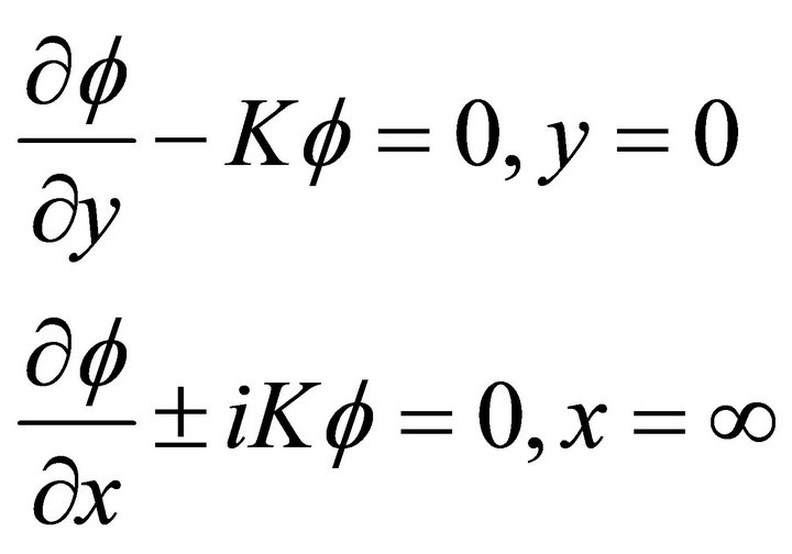 (2.2)
(2.2)
Here F is complex potential. On the free surface y = 0, velocity potential satisfies linear condition. We easy find its solution [12]:
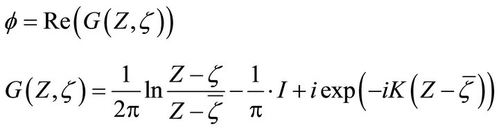 (2.3)
(2.3)
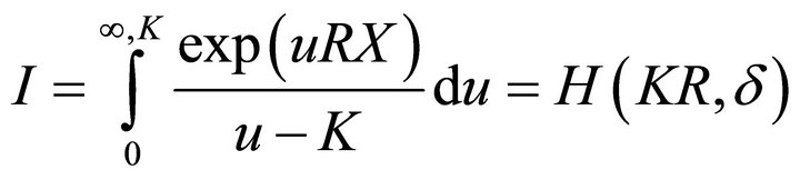
Here  is called green function, I is principle value integration of below
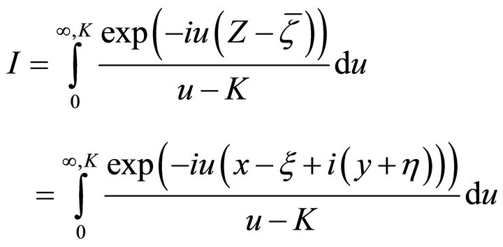
where the integral lower limit is 0, The integral upper limit is ¥,  is zero point of denominator, upper subscribe (¥, K) shows that it is principle value integration at point
 . From the expression of integration, the value I is determined by the parameters of K,
  ,
, . Let unit transfer as
 (2.4)
(2.4)
The principle value integration may be written as
 (2.5)
(2.5)
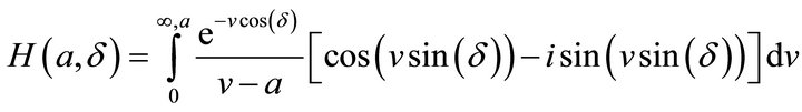
where  is called H-function with two parameters:
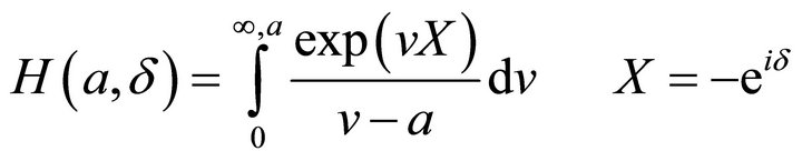 (2.6)
(2.6)
here parameters take value as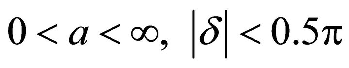 .
.
3. Intrinsic Properties
First, confirm that you have the correct template for your paper size. This template has been tailored for output on the custom paper size (21 cm × 28.5 cm).
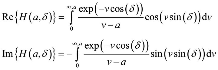
Let Re(H) and Im(H) are real part and imaginary part of  respectively. We will discuss Re(H) and Im(H) with parameters a and d.
3.1. Parameter ( = 0
In the case d = 0, from expression of , we easy know, Im(H) = 0, and
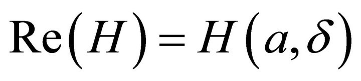 , or
, or
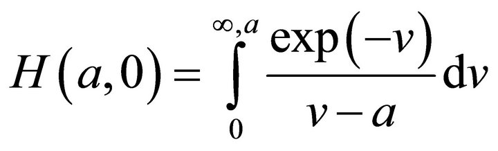 (3.1)
(3.1)
Above formula is principle value integration with one parameter, and may be rewritten as:
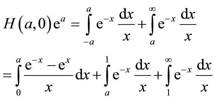
We easy obtain
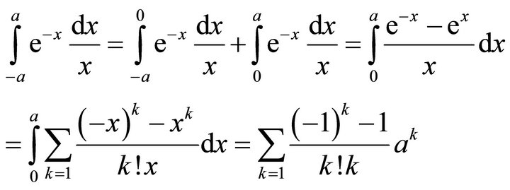
And by adopting subsection integration method, we have:
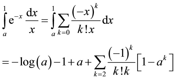 (3.2)
(3.2)
So that:
Here constant is:
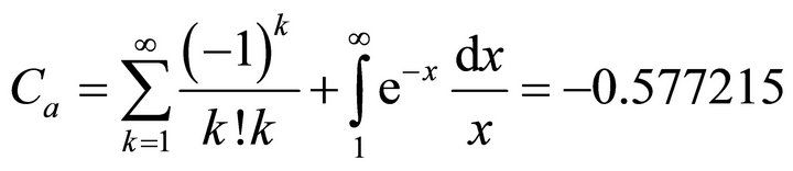 (3.3)
(3.3)
At last, we have
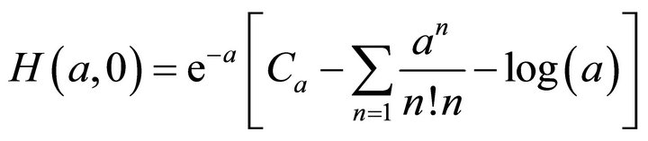 (3.4)
(3.4)
The integral value of H(a,0) is shown in Figure 1. From Figure 1, we have below theorem:
Theorem 1. 1)  as
as .
.
2)  as
as .
.
3) The lowest value 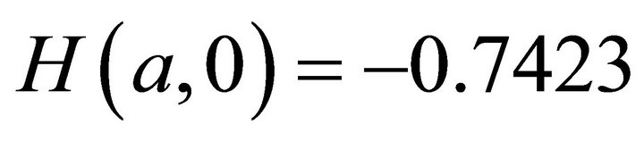 when a = 1.347.
4) On the domain , the curve is down.
5) On the domain , the curve is rise.
3.2. Parameter ( ( 0
If the value of parameters d is not zero, we have
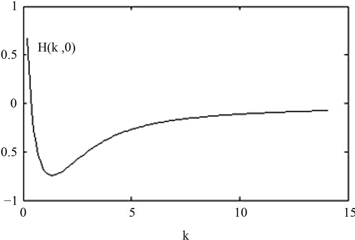
Figure 1. One parameter principle value integration H(a, 0).
And:
 (3.4)
(3.4)
From above formula, we have below theorem:
Theorem 2. The real part of function  is Symmetric function, or
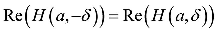 . The imaginary part of
  is antisymmetric function, or
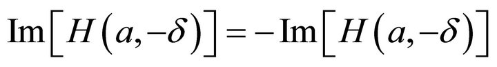 ;
;
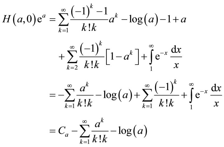
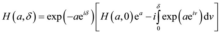
By using expression of Green function, we have ordinary equation:
So that we may express Green function as:
Using series expansion, we get:
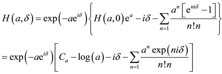 (3.5)
(3.5)
Here constant Ca = −0.577215. It is easy to calculate H-function by using above formula with given parameters. The numeric results are shown in Figures 2 and 3.
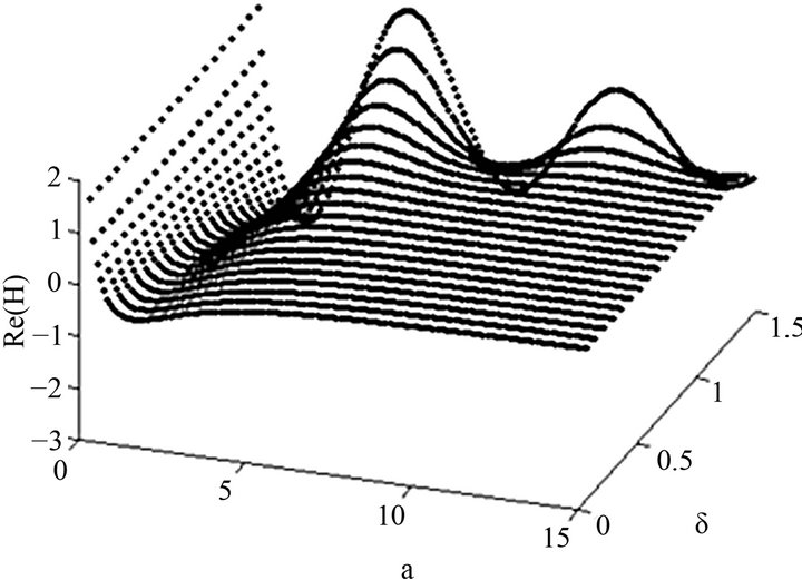
Figure 2. Real part Re(H) varied with parameters.
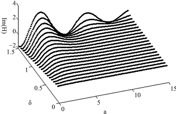
Figure 3. Imaginary part Im(H) varied with parameters.
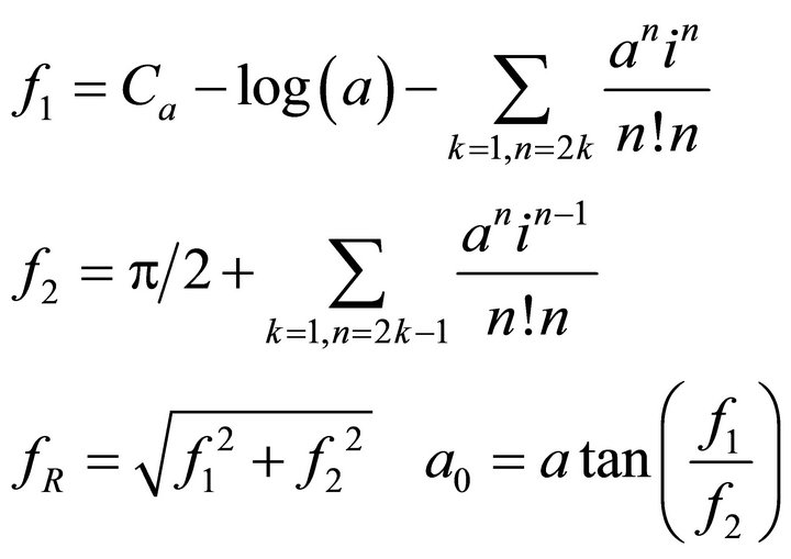
3.3. Property of ( = (/2
Considerd = p/2, then H-function may be written as:
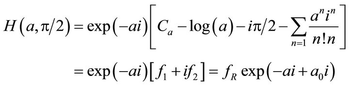 (3.7)
(3.7)
Here
4. Properties of Green Function
By using expression of H-function, we have below theorem:
Theorem 3. Consider field point  and source point
  are below free surface, the Green function may be expressed as:
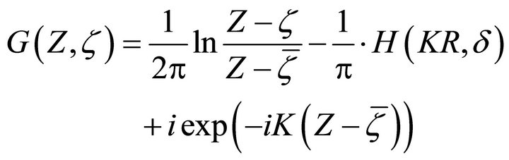 (4.1)
(4.1)
Here
 (4.2)
(4.2)
where constant Ca = –0.577215.
4.1. Vertical Line
Consider field point  and source point ζ = ξ + iη take value at vertical line
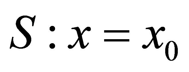 ,
, . According to the define of X, we have X = –1, or d = 0. In this case, the Green function is
 (4.3)
(4.3)
From above formula, last term is imaginary part of Green function, others at right is real part. Above formula also show that the Green function may represented by using H-function at d = 0.
4.2. Horizontal Line
Consider field point 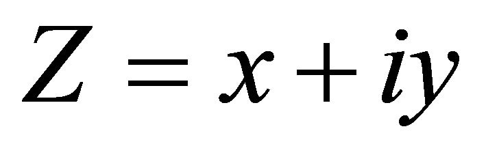 and source point ζ = ξ + iη take value at horizontal line S:
 ,
, . According to the define of X, we have
  . In this case, the Green function is
 (4.4)
(4.4)
Here
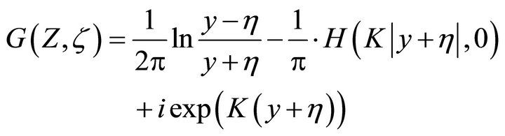
On the free surface, y0 = 0, X = ±i. Consider X = –i, or δ = π/2, the Green function can be written as:
 (4.5)
(4.5)
On the free surface, the Green function may represented by using H-function at .
.
5. Derivation of Green Function
We know, the derivation of potential are:
 (5.1)
(5.1)
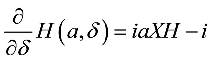
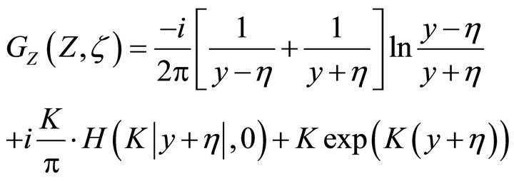
It is easy to obtain the derivation of Green function as:
 (5.2)
(5.2)
Consider field point  and source point ζ = ξ + iη take value at vertical line S:
 ,
,  , we have formula of two parameter
 :
:
6. Conclusion
In the paper, the Green function is simplified from integral formula by using two parameters. The intrinsic properties of Green function are discussed on vertical line and horizontal line. The derivation of Green function is obtained by using complex theory.
REFERENCES
- P. Andersen and W. Z. He, “On the Calculation of TwoDimensional Added Mass and Damping Coefficients by Simple Green’s Function Technique,” Ocean Engineering, Vol. 12, No. 5, 1985, pp. 425-451. doi:10.1016/0029-8018(85)90003-4
- J. V. Wehausen and E. V. Latoine, “Surface Waves,” In: S. Flügge, Ed., Encyclopedia of Physics, Springer, Berlin, 1960, pp. 446-778.
- A. H. Clement, “An Ordinary Differential Equation for the Green Function of Time-Domain Free-Surface Hydrodynamics,” Journal of Engineering Mathematics, Vol. 33, No. 2, 1998, pp. 201-217. doi:10.1023/A:1004376504969
- N. Kuznetsov, V. Maz’ya and B. Vainberg, “Linear Water Waves: A Mathematical Approach,” Cambridge University Press, Cambridge, 2002.
- J. N. Newman, “Algorithm for the Free-Surface Green Function,” Journal of Engineering Mathematics, Vol. 19, No. 1, 1985, pp. 57-67.
- H. Shen, “Computational Method of Surface Green Function with No Numerical Integration,” Journal of Dalian institute of Technology, Vol. 17, No. 1, 1988, pp. 75-84.
- Q. B. Zhou, G. Zhang and L. S. Zhu, “The Fast Calculation of Free Surface Wave Green Function and Its Derivatives,” Chinese Journal of Computational Physics, Vol. 16, No. 2, 1988, pp. 113-119.
- C. Yang, F. Noblesse and R. Löhner, “Comparison of Classical and Simple Free-Surface Green Functions,” Journal of Offshore and Polar Engineering, Vol. 14, No. 4, 2004, pp. 256-264.
- L. Shen Liang, et al., “A Practical Numerical Method for Deep Water Time Domain Green Function,” Journal of Hydrodynamics A, Vol. 22, No. 3, 2007, pp. 380-386.
- F. John, “On the Motion of Floating Bodies I,” Communications on Pure and Applied Mathematics, Vol. 2, 1949, pp. 13-57.
- F. John, “On the Motion of Floating Bodies II,” Communications on Pure and Applied Mathematics, Vol. 3, 1950, pp. 45-101.
- Y. Z. Liu and G. P. Miu, “Theory of the Motion of Ships in Waves,” Shanghai Jiao Tong University Press, Shanghai, 1987.
- R. Hein, M. Duran and J.-C. Nedelec, “Explicit Representation for the Infinite-Depth Two-Dimensional Free-Surface Green’s Function in Linear Water-Wave Theory,” SIAM Journal on Applied Mathematics, Vol. 70, No. 7, 2010, pp. 2353-2372. doi:10.1137/090764591
- W. D. Kim, “On the Harmonic Oscillations of a Rigid Body on a Free Surface,” Journal of Fluid Mechanics, Vol. 21, No. 3, 1965, pp. 427-451.
- M. D. Greenberg, “Application of Green’s Functions in Science and Engineering,” PrenticeHall, Englewood Cliffs, 1971.
- C. Macaskill, “Reflexion of Water Waves by a Permeable Barrier,” Journal of Fluid Mechanics, Vol. 95, No. 1, 1979, pp. 141-157.
- R. Dautray and J. L. Lions, “Analyse Mathématique et Calcul Numérique Pour les Scienceset les Techniques,” Vol. 2, Masson, Paris, 1987.
- C. F. Liu, et al., “New Convolution Algorithm of Time—Domain Green Function,” Journal of Hydrodynamics A, Vol. 25, No. 4, 2010, pp. 25-34.
- N. Kuznetsov, V. Maz’ya and B. Vainberg, “Linear Water Waves: A Mathematical Approach,” Cambridge University Press, Cambridge, 2002.
- C. C. Mei, M. Stiassnie and D. K.-P. Yue, “Theory and Applications of Ocean Surface Waves, Part 1: Linear Aspects,” World Scientific, Hackensack, 2005.
- J. V. Wehausen and E. V. Latoine, “Surface Waves,” In: S. Flügge, Ed., Encyclopedia of Physics, Vol. IX, Springer, Berlin, 1960, pp. 446-778.
- R. Harter, I. D. Abrahams and M. J. Simon, “The Effect of Surface Tension on Trapped Modes in Water-Wave Problems,” Proceedings of the Royal Society of London Series A: Mathematical, Physical and Engineering Science, Vol. 463, No. 2, 2007, pp. 3131-3149.
- R. Harter, M. J. Simon and I. D. Abrahams, “The Effect of Surface Tension on Localized Free-Surface Oscillations about Surface-Piercing Bodies,” Proceedings of the Royal Society of London Series A: Mathematical, Physical and Engineering Science, Vol. 464, No. 2, 2008, pp. 3039-3054.
- O. V. Motygin and P. McIver, “On Uniqueness in the Problem of Gravity-Capillary Water Waves above Submerged Bodies,” Proceedings of the Royal Society of London Series A: Mathematical, Physical and Engineering Science, Vol. 465, No. 3, 2009, pp. 1743-1761.
NOTES
*The paper is financially supported by China national natural science foundation (No. 51139005), and (No. 51279149) and China national education department doctoral foundation (No. 20120143130002).
#Corresponding author.