Journal of Environmental Protection
Vol. 4 No. 7A (2013) , Article ID: 34708 , 16 pages DOI:10.4236/jep.2013.47A010
SWAT Model Prediction of Phosphorus Loading in a South Carolina Karst Watershed with a Downstream Embayment
![]()
1Center for Forested Wetlands Research, USDA Forest Service, Cordesville, USA; 2Department of Civil, Architectural, and Environmental Engineering, North Carolina A&T University, Greensboro, USA; 3Baruch Institute of Coastal Ecology and Forest Science, Clemson University, Georgetown, USA; 4Florida A&M University, Tallahassee, USA.
Email: damatya@fs.fed.us
Copyright © 2013 Devendra M. Amatya et al. This is an open access article distributed under the Creative Commons Attribution License, which permits unrestricted use, distribution, and reproduction in any medium, provided the original work is properly cited.
Received June 1st, 2013; revised July 3rd, 2013; accepted July 13th, 2013
Keywords: Water Quality Models; Lake Marion; Runoff; Groundwater (Baseflow); Losing Streams; Deep Percolation; Settling Rate
ABSTRACT
The SWAT model was used to predict total phosphorus (TP) loadings for a 1555-ha karst watershed—Chapel Branch Creek (CBC)—which drains to a lake via a reservoir-like embayment (R-E). The model was first tested for monthly streamflow predictions from tributaries draining three potential source areas as well as the downstream R-E, followed by TP loadings using data collected March 2007-October 2009. Source areas included 1) a golf course that received applied wastewater, 2) urban areas, highway, and some agricultural lands, and 3) a cave spring draining a second golf course along with agricultural and forested areas, including a substantial contribution of subsurface water via karst connectivity. SWAT predictions of mean monthly TP loadings at the first two source outlets were deemed reasonable. However, the predictions at the cave spring outlet were somewhat poorer, likely due to diffuse variable groundwater flow from an unknown drainage area larger than the actual surface watershed, for which monthly subsurface flow was represented as a point source during simulations. Further testing of the SWAT model to predict monthly TP loadings at the R-E, modeled as a completely mixed system, resulted in their over-predictions most of the months, except when high lake water levels occurred. The mean monthly and annual flows were calibrated to acceptable limits with the exception of flow over-prediction when lake levels were low and surface water from tributaries disappeared into karst connections. The discrepancy in TP load predictions was attributed primarily to the use of limited monthly TP data collected during baseflow in the embayment. However, for the 22-month period, over-prediction of mean monthly TP load (34.6 kg/mo) by 13% compared to measured load (30.6 kg/mo) in the embayment was deemed acceptable. Simulated results showed a 42% reduction in TP load due to settling in the embayment.
1. Introduction
In recent years there has been an increasing demand for the sustainable management of water quantity and water quality of various water bodies such as streams, lakes, reservoirs, and groundwater throughout the nation. Diffuse pollution from urban stormwater and agricultural runoff are among the leading causes of water pollution in the USA [1]. The 2000 National Water Quality Inventory (NWQI) reported that nutrients were the leading pollutants in lakes and reservoirs, the fifth in rivers and streams and the eleventh in estuaries [2]. The nutrients nitrogen (N) and phosphorus (P) stimulate the growth of a variety of types of aquatic plants resulting in eutrophication and impairment in the beneficial uses of water bodies [3]. Section 303(d) of the Clean Water Act (CWA) and the US EPA Water Quality Planning and Management Regulations require that states identify, list, and prioritize those water bodies that are impaired for various uses such as drinking, swimming, aquatic habitat etc. and develop Total Maximum Daily Loads (TMDLs) for the pollutants of concern [4].
Chapel Branch Creek (CBC) is a small tributary of Lake Marion located within the Santee River/Lake Marion Sub-Basin, HUC 03050111-010 [5] (Figure 1). Although a small portion of the subbasin (1555 ha of 90,360 ha), CBC has high growth potential primarily due to Lake Marion access with many recreational activities such as fishing, boating, swimming, and camping [5] as well as many new lakeside residential subdivisions. The watershed was included on the 2008 303(d) list of impaired water bodies for impairment of aquatic life (AL) by total phosphorus (TP) and pH [6]. Since hydrology is often a primary driving force for understanding nutrient loading dynamics and its subsequent downstream water quality impacts, TMDL estimations for TP were developed for CBC by the US Forest Service with aid by Clemson University and the State Public Service Authority
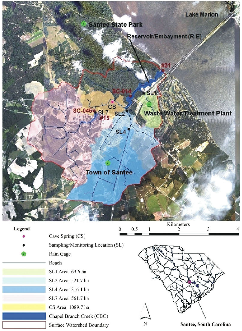
Figure 1. Location map showing boundary and tributaries of Chapel Branch Creek watershed draining to Lake Marion, SC. Rain gauges and flow monitoring (sampling) stations are shown (After [27]).
(Santee Cooper) by employing a monitoring, and modeling approach for pollutant load quantification and subsequent source area identification [7]. Both the monitoring and modeling approaches provided a better understanding of the hydrologic and nutrient cycling and transport (flow pathways) processes on the watershed of interest. Potential effects of karst features and interactions with Lake Marion level on hydrology and potential flow paths of the CBC watershed have been recently discussed by [8,9].
There are a large number of predictive models in the literature that vary from simple lumped parameter to physically-based complex models capable of simulating various management practices in varying temporal and spatial scales [10-12]. [13] developed multiple regression models relating land use categories of agriculture, forest, urban, and wetland areas that comprise a lower portion of the Lake Marion drainage to in-stream concentrations of total N and total P in eight, low-order watersheds. The authors found a greater predictive strength for the N models explaining more variability of stream nutrient concentration than that for the P models, likely reflecting differing pathways from terrestrial to aquatic systems. [14] also used the WASP5 (Watershed Analysis and Simulation Program 5) lake water quality and hydrodynamic modeling system for simulating water quality of Lake Marion itself comprising of 330.7 km2 surface area using data from 1985-1990. The authors calibrated the hydrodynamic model with the estimates of daily lake volume and the water quality model was calibrated to various nutrients and other water quality parameters. Similarly, [15] used a comprehensive modeling approach that linked SWAT with the WASP model for water quality assessment and management or a reservoir with 133.5 km2 surface area in Texas.
Based on various applications of three models (SWAT, HSPF, and DWSM), [16] reported that SWAT and HSPF were found suitable for predicting annual flow volumes, sediment and nutrient loads, although monthly predictions were generally good, except for months having extreme storm events and hydrologic conditions. Some other studies showed a good correlation and model efficiency in predicting monthly P loadings using the SWAT model [17-19].
Although in recent years the SWAT model has been widely and successfully tested for various geographical regions with multiple management practices, studies on watersheds affected by karst features (e.g. sinkholes, losing streams, springs, and caves that potentially provide for significant groundwater linkages) are limited. These limitations can be due to the complex processes by which groundwater can variably influence surface water flow, both in magnitude and duration, as well as flow paths complicating the model calibration, thus requiring the use of more complex subsurface models [20-23]. Reference [24] also reported that modeling of groundwater flow in karstic aquifers has been less successful and more work should be conducted in this area, including all types of interactions, as well as determining specific processes and mechanisms for contaminant transport. Recently, [25] modified the SWAT 2005 code to simulate faster aquifer recharge in karst environments (SWAT-B&B) by modifying subroutines for deep groundwater recharge and maximizing the hydraulic conductivity for sinkholes simulated as ponds and for losing streams and tributaries. The authors concluded that the SWAT model can be used to simulate the frequency of occurrence of pollutant concentrations and daily loads. Yachtao [26] modified the works of (SWAT-B&B) in SWAT-Karst to represent karst environments at the hydrologic response unit (HRU) scale. Accordingly, in the Opequon Creek watershed study, [26] found that a SWAT-Karst model that used the HRU to represent sinkholes had a more notable impact in the watershed hydrology than SWAT-B&B using a pond to represent sinkholes; the author reported that the SWAT-karst and the SWAT-B&B version performed better than the SWAT alone for predicting streamflow in a karst-influenced watershed. Most recently, [27] used the SWAT model to simulate the monthly streamflow pattern and dynamics of the karst affected CBC watershed tributaries and its embayment adjacent to Lake Marion, water levels of which dynamically influence the hydrology and water quality of the CBC system [8,9]. Results demonstrated the substantial influence on the water balance of the karst features with conduit and diffuse flow as an explanation [9] for the missing upstream flows appearing via subsurface conveyance to the downstream cave spring [8] providing a more accurate simulation at the embayment outlet [27]. Results also highlighted influences of downstream lake levels and karst voids/conduits on the watershed hydrologic balance [9]. The nutrient loadings and their patterns of the CBC watershed as affected by the karst and lake water levels, however, have not yet been fully described for this karst watershed.
The main objective of this study is to test the capability of the operational SWAT2005 model to predict mean monthly total phosphorus (TP) loadings at three major tributaries of the CBC watershed affected by karst features with a minimum calibration, as well as at the overall TP concentrations and loadings at the downstream reservoir-embayment (R-E) outlet. This study provided an opportunity to test the SWAT model’s simple approach of completely mixed system and simple settling rate to predict TP loadings at the R-E embayment downstream at the lake edge instead of using other complex eutrophication model like WASP [28] applied by [14] for simulating the water quality of Lake Marion.
2. Materials and Methods
2.1. Site Description
Chapel Branch Creek (CBC) is a small tributary of the former Santee River that now flows directly into Lake Marion, a dam reservoir, near the town of Santee, SC, USA (a portion of the 11 digit HUC 03050111-010) (Figure 1). The watershed with its main outlet at the lake (33˚30′7.5″N and 80˚27′37.1″W) drains approximately 1555 ha of land through two main drainage areas (Figure 1).
Topography of the watershed is characterized by flat lands at approximately 37 m above mean sea level in the upstream areas with somewhat steeper topography (25 to 30 m) on the downstream section near Lake Marion. The watershed also contains features of karst topography, such as losing streams, sinkholes, springs, and caves. These features are due to the ongoing dissolution of the underlying Santee Limestone, which influences both surface and ground water storage and flow [9]. The Santee Limestone (SL) is part of the northern end of the Floridan Aquifer system, and a major groundwater aquifer in coastal South Carolina for industrial, agricultural, and public purposes [29]. The SL unit in the CBC watershed located at the northern portion of the Floridan aquifer contributes to the groundwater primarily as a diffuse discharge [30].
The watershed is comprised of complex land use patterns with residential, commercial, and industrial areas interspersed among agricultural and forested lands and has two main drainage areas. The north-western area with some forests and croplands is the valley of CBC, which is a natural creek that has been modified by drainage ditches near the watershed boundary and a dam and a pond just downstream of a golf course within the valley [31]. The south-eastern section is primarily ditches, culverts and storm drains associated with the development along Interstate 95 and SC Highway 6 and some croplands.
Two major tributaries (CS and SL2) and one small tributary (SL1) drain to the downstream reservoir-like embayment (R-E) of the CBC watershed. The cave spring (CS) outlet drains a surface watershed of approximately 1090 ha comprised of agricultural and forested lands and also a golf course, besides groundwater from an unknown area of (Figure 1). The second tributary at SL2 outlet drains approximately 550 ha of land comprised of an urban municipal area along with major highways and roads, and some agricultural and forested lands. A third small tributary draining approximately 63 ha at SL1 contains another golf course that received wastewater treatment plant effluent via land application.
Agriculture has been historically the primary land use in the watershed with small grain and vegetables as the major produce from the area. Most of the forested lands are located within Santee State park on the northwest left bank of the CBC [32]. More details of the site, land use, and soils can be found elsewhere [33].
2.2. Hydrologic Monitoring
Rainfall was continuously measured from August 2006 to October 2009 with varying periods at three installed automatic and manual gauges at the town of Santee (TS) (from August 2006 to October 2009), Wastewater Treatment Plant (WWTP) (from March 2007 to October 2009), and Santee State Park (SSP) (from May 2007 to October 2009) (Figure 1). Daily rainfall data from these three rain gauges from 2006 to 2009 were used in the SWAT model simulations. Data on air temperature, relative humidity, solar radiation, and wind speed were obtained from the nearby US Fish and Wildlife Service (US FWS) weather station (http://fam.nwcg.gov/fam-web/) at Santee National Wildlife Refuge across Lake Marion to the northeast to estimate daily PET using Turc’s method [34] as described by [35]. Details of rainfall measurements and analysis are discussed in [27]. Streamflow rates were measured using Isco® (Lincoln, NE) flow meters at the outlets of three major tributaries: SL1, SL2, and CS. In this study, data measured from August 2008 to July 2009 at SL1, July 2007 to July 2009 at SL2 and January 2009 to October 2009 at the cave spring (CS) were used for analysis. Details of data processing and quality control for all flow data are presented in [7,27].
2.3. Water Quality Sampling
Manual (grab) sampling of storm events was performed at each of the three major stream tributaries (SL1, SL2, and CS). Each location was sampled with five grab samples and one field duplicate for one storm event in each of the four seasons (fall (September-November: November 11, 2009), winter (December-February: February 22, 2008), spring (March-May: April 02, 2009), summer (June-August: July 29, 2009)). Samples were immediately preserved on ice and taken to the South Carolina Department of Health and Environmental Control (SCDHEC)-certified Santee Cooper Analytical and Biological Laboratory (Moncks Corner, SC for all analyses of nutrients including Phosphorus (P). Samples were analyzed for TP using the colorimetric, Semi-Automated Digester, Atomic Absorption II (AAII) methods (EPA Method 365.4) [36]. An Isco® discrete water quality sampler was connected to the Isco® flow logger at both SL1 and SL2 stations, which was programmed to trigger the sampler on flow-proportional basis capturing both large events and small base flows. A 3rd Isco® sampler connected to an Infinities® (Port Orange, FL) logger at the CS outlet was programmed based on 2-hour time interval during the flow events. Laboratory analyses were performed for P using the same techniques as previously described for grab samples. Automatic sampling was conducted for varying periods between July 2007-July 2009 at SL2, October 2008 to October 2009 at SL1 and January-October 2009 at CS at these three stations. Continuous flow data and the P concentrations measured by discrete sampling by Isco at various download intervals were used to obtain the P load for a given interval at each of the stations. Loads at various intervals were summed to obtain the monthly and annual loads. Details of water quality sampling, laboratory analysis, flow measurement, and load calculation methods are described in [7,8].
2.4. SWAT2005 Model
A distributed, watershed-scale hydrology and water quality model based on SWAT (Soil and Water Assessment Tool) [12] was created for the CBC watershed (Figure 1). The model was developed to predict the impact of land management practices on water, sediment, and agricultural chemicals in complex watersheds with varying soils, land uses and management conditions [37-39] and further for the TMDL development [19,40-41].
2.5. Phosphorus Processes in SWAT
SWAT can estimate HRU-level phosphorus (P) concentrations, which are summed at the subwatershed level; the losses are routed through channels, ponds, wetlands, depressional areas, and/or reservoirs to the watershed outlet. The model comprehensively simulates transfers and internal cycling of the major forms of P, similar to how it simulates N without gas-phase transitions [42]. The P-cycle is complex and appears to be better understood and modeled. Soluble organic P is recognized as being important in many natural ecosystems [42]. Soluble phosphorous (P) loss in surface runoff is based on partitioning P between the solution and sediment phases [43], and is predicted using the labile P concentration in the top soil layer, runoff volume, and a partitioning factor. Sediment transport of P is simulated using a loading function similar to organic N transport [44]. Initial nutrient levels can be input as concentrations; however, all calculations in SWAT are performed on a mass basis. Instream nutrient transformations are based on a QUAL- 2E model [45] with components algae (as chlorophyll-a), dissolved oxygen, carbonaceous oxygen demand, organic P, and soluble P. In this study, the SWAT model only, with its active in-stream components, was applied without linking it to another water quality model like QUAL- 2E. White [46] found no significant improvement concerning simulated monthly TP yields from their study watershed by adding the detailed in-stream QUAL2E model to the SWAT. Details of all the hydrologic and nutrient processes (e.g. surface runoff, base flow, water yield, ET, components of N and P etc.) including the flow and nutrient routing simulated by SWAT and the output variables (water, sediment, nutrients, and pesticides) can be found in [47].
2.6. SWAT Model Setup for Tributaries and Reservoir Embayment (R-E)
In order to apply the SWAT model for scientifically valid determination of the nutrient loadings from various source areas determined by land uses and management practices, the model must first be tested for its ability to predict the hydrology component (runoff or stream flow) that drives these loadings. The same model setup in a companion study [27] for the SWAT calibration and validation for flows in the CBC watershed was used in this study as well. Accordingly, the CBC watershed was first divided into 31 subwatersheds (Figure 2).
Each subwatershed was parameterized using GISbased spatial data on watershed characteristics such as topography, soils, land use, hydrography, and land and crop management practices. The downstream embayment (R-E) on CBC was assumed as a reservoir on subwatershed 31. Similarly, a golf course pond, an impoundment upstream of CBC at SL7, was also represented by a 2nd reservoir added to subwatershed 15 (Figure 1). The final outlet (31) for Chapel Branch Creek was at its downstream boundary of the reservoir-like embayment (R-E) at Lake Marion (Figure 1). A point source was then added in the subwatershed 16 with a cave spring (CS), which contributes a sustained groundwater flow possibly from an estimated area of 1090 ha or more, including SL2 and SL7 subwatersheds, to the CBC headwaters. The CS flow was substantially higher than the flow measured at the other tributaries, strongly indicating a significant water loss from the surface watershed to subsurface flow from SL1 and SL2 subwatersheds, possibly in dissolution channels associated with the karst features of this watershed [8] or due to added subsurface flow with an effective area larger than the surface watershed.
Both the precipitation and weather (for estimating potential evapotranspiration) data measured between March 2007 and October 2009 were used as inputs to calibrate runoff (stream flow) from three main tributaries (source areas) of the CBC watershed. Since the TMDL was to be developed for the SC014 station in the middle of flooded portion of the downstream stem of the CBC (e.g. R-E) at the edge of Lake Marion (Figure 1), the distributed model was also tested for its ability to predict the flows and nutrient concentrations and loadings measured during March 2007 to October 2009 at this outlet location. Details of the model setup with GIS spatial data on DEMs, land use/land cover, soils, and hydrography of the CBC watershed and temporal data from rain gauges and
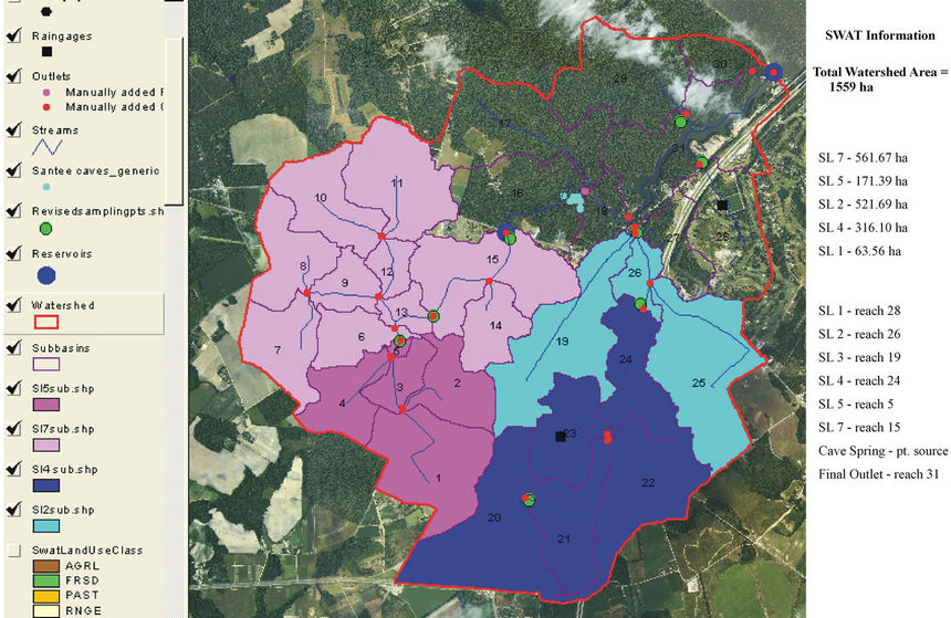
Figure 2. Delineation of CBC watershed into 31 subbasins and stream tributaries.
weather station have been published elsewhere [27].
2.7. Model Parameterization
The GIS spatial data on the USGS 1:24,000 scale DEM, land use in the SWAT built by digitizing digital USGS topographic maps and 2005 National Agricultural Imagery Program (NAIP) aerial photography with 1 m resolution, the SSURGO shapefile, and database for the SC-075 soil map of Orangeburg County, South Carolina obtained from the USDA-NRCS website were analyzed and processed to obtain the necessary spatial layers for the SWAT-CBC model setup [32,33,48]. Detailed parameterization for hydrologic calibration and validation of the SWAT model for the CBC watershed was described by [27]. The authors noted that calibration of the SWAT model constructed for the CBC watershed was more than a standard calibration due to complex karst watershed characteristics including depressions and sinkholes. These karst features can reroute surface waters from these tributaries to the underground system through interconnected conduits as was shown by [9]. Measured flow data at SL2 and its upstream area SL4 (Figure 1) suggested that a substantial portion of surface water might have been lost to the groundwater and that potentially reappeared at the CS as shown by [8,9]. Accordingly, [27] used high soil conductivity values both for the land surface as well as tributaries to make the model lose water as was done by [25]. Similarly, a high value of the deep percolation coefficient was used in the model to allow loss of extra surface water from the system to the deep aquifer mimic the effects of karst features like sink-holes, depressions, and losing streams. The most sensitive hydrologic parameters in flow calibration for this karst watershed included curve number, effective hydraulic conductivity in the main and tributary alluvium, and the deep aquifer percolation coefficient [27].
In this section parameterization for total phosphorus (TP) as the nutrient of concern is discussed. Besides the flow rates, the depth and accuracy of nutrient calibration is also dependent on the information available, such as fertilizer usage rates, initial soil nutrient concentrations, loss rates, and types of crops grown, and other land use and crop management practices. Methods suggested in [11,25,49] were followed for parameterizing the CBC watershed as needed.
The SL1 and SL2 subwatersheds contain mostly agricultural land (AGRL), golf courses resembling the range (RNGE), Transportation (UTRN), and Commercial (UCOM) landuses. For agricultural land use, the dominant crops in the watershed were vegetables-green beans, soy beans, wheat, corn, peanuts, and collard greens based on interviews with town employees and visual field observations. The SWAT land use code for row crops (AGRL) and its default values were used for modeling the HRUs with agriculture land use. At least one planter grew different vegetables three times a year, but exact dates for planting were unknown. Similarly, exact fertilizer compositions were unknown. This made itemization of agricultural lands difficult, so assumptions had to be made for management practices. The fertilizer chosen from 54 default fertilizer types in the SWAT database was 00-06- 00. For the AGRL land use, this fertilizer was applied twice annually after planting on April 1 and July 3. The crops were assumed harvested twice annually, on July 1 and October 1. Exact fertilization rates at two golf courses on the site were also unknown, but it was assumed that fertilizer would be applied during the summer months. The subwatershed draining SL1 station (Figure 1) contains a Wastewater Treatment Plant that irrigates a golf course with its effluent application. The treatment plant had data for the discharge rates and schedule as well as nitrogen (N) concentration data, but no data for phosphorus (P) in effluent. However, the fractions on N and P (0.71 and 0.29) found in the literature [50] were used to obtain P fraction using the N data.
Parameters used in the TP calibration for basin-wide application included the phosphorus percolation coefficient (PPERCO), and the phosphorus soil partitioning coefficient (PHOSKD). The selected values (Table 1) were identical to those reported by [15,39] for PPERCO and by [51] for PHOSKD. The default value used for the phosphorus availability index (PSP) was obtained from either from the SSURGO soil or SC Orangeburg County soil survey report. Sediment related parameters were not calibrated and only default values were used since the measurement data were not available.
Nutrient inputs were defined as a point source in subwatershed # 16 to represent Cave Spring (CS) (Figure 1), which contributed a sustained groundwater flow as previously discussed. For a point source, SWAT requires inputs in the form of soluble mineral and organic P instead of TP. This separation was not defined by available mea-
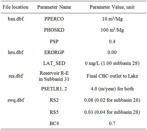
Table 1. Input parameters used in SWAT for Total Phosphorus (TP).
sured data, so it was assumed that the proportions were the same as observed in the measured data at SC014 (by Santee Cooper Authority) or 58% organic P and 42% mineral P of TP. Based on the limited additional water quality data collected at the surface stream (SS) inlet from upstream SL7 to the CS and the adjacent groundwater (GW) source linked to the CS outlet, the bulk amount of sediment seems to have been transported to the CS outlet from the SL7 and its downstream section to SS location [9].
The options of in-stream water quality and Algae/ CBOD modeling were made active in the model. Sensitive parameters for in-stream water quality were sediment source rate for dissolved phosphorus (RS2), organic phosphorus settling rate (RS5), and the rate constant for mineralization of organic P to dissolved P (BC4). Additionally, the effect of sediment transport for phosphorus loading was accomplished through various sedimentrelated model parameters. Such parameters include phosphorus enrichment ratio (ERORGP), coefficients for sediment channel routing (SPCON and SPEXP), channel erodibility factor (CH-EROD), and channel cover factor (CH_COV). Values chosen for final model calibration are shown in Table 1.
2.8. Reservoir Parameterization
In addition to subwatershed simulations, the downstream section of CBC near Lake Marion was modeled as a reservoir that receives discharge from the outlets of CS, SL1, and SL2, and some minimal flow from the forest with subwatersheds # 16, 17, 18, 29, 30, and 31) on the northwest bank (Figure 2) which was modeled using SWAT default parameters. The final reach of this watershed at subwatershed outlet 31 (Figure 1) was designated as a reservoir during the SWAT watershed delineation. The CBC impairment for TP, Chlorophyll-a, and pH parameters at SC014 in subwatershed 31 (Figure 1) was listed by SCDHEC based on long-term data monitored by Santee Cooper Authority. Since this portion of the CBC is an embayment of Lake Marion, the best method to evaluate the impact of loading at SC014 was to estimate the residence time and potential nutrient removal of water from all three sources in the CBC embayment. Since this CBC embayment is much smaller (surface area = 0.154 km2 and 9.8 × 10⁴ m3 volume at maximum lake level; [8]) than the Lake Marion reservoir, the one-dimensional complete mixing model without lateral diffusion available in SWAT was assumed adequate for modeling nutrient levels in the embayment. SWAT incorporates a simple empirical model to predict the trophic status of the water body and makes the following assumptions for calculating the nutrient transformations [48]:
1) The shallow water-body (embayment) system is completely mixed. Nutrient inputs from three major sources (CS, SL1, and SL2) are instantaneously distributed throughout the embayment system.
2) Water stratification and intensification of phytoplankton in the surface waters are ignored.
3) Nutrient transformation is limited to the removal by settling only, ignoring transformation between the nutriaent pools.
To test the model’s ability to predict phosphorus (TP), water quality data from SC014 for 2007-2009 was used to find average monthly concentration values for organic P (RES_ORGP) and soluble P (RES_SOLP) in mg·L−1. The SC014 data was reported in ppm (mg·L−1) for these species: OPO4 and T-PO4 of total P. RES_ORGP was found by subtracting the OPO4 from TP (Total Phosphorus). Values for each species were then averaged and used as initial concentration input in the SWAT interface for reservoir (31). Reservoir settling velocity was an important and sensitive calibration parameter.
Although SWAT allows entering two settling values (PSETLR1, PSETLR2) for phosphorus for a year depending upon seasons, only one value (PSETLR) was used for the whole year. The default value for PSETLR is 5.0 m/year. A sensitivity analysis of the settling rate was conducted throughout its ranges in the SWAT model database. Chapel Branch Creek is a shallow water body with a history of sediment pollution. Although the SWAT manual [49] suggested values < 0 for shallow water bodies, calibration was only achieved with higher values. Values of −5, −2, (for export) 0, and 5 (for settling) showed the most sensitivity. Since the values of 5 and 10 both yielded the same results, a value of 4 for PSETLR was chosen for final analysis (Table 2). Data for SC014 also included Total Suspended Solids (TSS) results. The average TSS concentration in mg·L−1 was calculated and input as the reservoir’s RES_NSED parameter for equilibrium sediment concentration. All these values are given in Table 2.
Predicted total cumulative TP load exported out of the reservoir after accounting for losses due to settling in the reservoir were used to compare with the measured TP concentration at the downstream embayment (R-E) out-
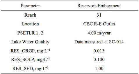
Table 2. Nutrient Parameters used in SWAT for reservoirembayment (R-E) at the outlet.
let. The SWAT simulated monthly TP load from the reservoir was divided by the simulated monthly volume of water leaving this reach (reservoir) to obtain the monthly flow weighted concentration for the R-E embayment at the SC014 location. The estimates of monthly TP loads at SC014 location were obtained by multiplying the monthly R-E embayment flow from a water balance approach with the monthly measured TP concentration at SC014 location in the embayment. The simulated and estimated annual loads were obtained by summing the monthly values. The water balance and hydrologic modeling calibration at this R-E outlet have been described in detail by [8,27].
2.9. Model Evaluation Criteria
The model was simulated for 2006 to 2009 with 2006 as one year “warm-up” period which was not used for model testing for TP loading. The actual testing was performed with limited data measured during various periods of 2007-2009 on one individual subwatershed (SL1) and two other locations (SL2 and CS) draining multiple subwatersheds, as was done in its previous hydrologic modeling testing [27]. The measured TP data from both the continuous sampling and seasonal event sampling were used for the model testing. Since earlier SWAT hydrologic model did not result in an acceptable calibration for monthly flows for this complex karst watershed but produced acceptable (within 11% error) results for mean monthly values [27], model testing for TP loading was also performed only on a mean monthly basis for those three locations. However, the model testing at the SC014 location in the reservoir-embayment outlet was performed on a monthly scale by comparing the predicted flowweighted TP concentration with the measured concentration (Figure 1). Predicted monthly and annual TP loads were also compared with corresponding estimated TP loads in the embayment [27]. The sum of the monthly TP loads input from all three subwatersheds SL1, SL2, and CS were also compared with the total TP load exported from the R-E outlet to evaluate the net losses predicted by the model in the embayment.
The mean bias or mean absolute error (MAE %) between the measured and simulated TP loads for a given period were used for the evaluation of the model performance as described in the current literature [11,19,52]. Coefficient of determination (R2), mean and standard deviation were also used to compare the correlation and the distribution between monthly measured and predicted nutrient loads.
3. Results and Discussion
3.1. Hydrologic Calibration
SWAT calibration results on monthly stream flows at three CBC tributaries e.g. SL1, SL2, and the CS outlet were reported by [27] for the same study period. The authors found poor results with monthly calibration at SL1 and SL2 primarily due to the effects of losing waters on this karst watershed and their seasonal interactions with lake water levels as recently reported by [9]. Continuous flow measurements revealed that less than 10% of the rainfall was being produced as surface runoff particularly at SL1 outlet with negligible baseflow) and also at SL2 (with a small base flow) outlet [8]. The authors reported that the small amount of rainfall mostly as surface flow at these tributaries and the substantially larger flow (~ 60% of the rainfall) at the cave spring (CS) indicated a significant water loss from the surface watershed to subsurface flow or a groundwater source area substantially larger than the surface watershed. This subsurface source was also shown to be the dominant input to the flooded embayment in the lower section of CBC [8]. The monthly stream flows at SL1 and SL2 locations, both with multiple land uses, were over-predicted when lower lake levels were prevalent, suggesting surface water flow to groundwater (losing streams). The model under-predicted the flows during rising lake levels likely due to high conductivity and also a deep percolation coefficient representing flow lost to shallow and deep groundwater, respectively. However, the mean monthly flow calibration excluding data from large wet events in each of these three locations was reported to be acceptable (within 11% error).
3.2. TP Prediction at Stream Tributaries
3.2.1. SL1 Outlet
It was assumed that most of the TP component at the SL1 tributary is washed off as organic P with the sediment driven by the surface runoff for this flashy watershed. Simulated results showed that the TP loading at SL1 was dominated by sediment bound organic P, which mostly depends on the high runoff. For example, for a 10-month period in 2009, the simulated organic P leaving subbasin SL1 was 27.5 kg compared to negligible (0.03 kg) amount of soluble P. These predictions may be reasonable as this subwatershed yielded rapid peaks and short duration hydrographs [7] with barely any base flow compared to the SL2 station discussed below. The difference between the mean monthly predicted and measured TP load for the 12-month period from September 2008 to August 2009 was 0.5 kg over-prediction (Figure 3(a)). However, when the data of October 2008 and April 2009 with very large storm events were removed (Figure 3(b)), the difference between the mean monthly predicted and measured data was reduced to 0.3 kg. This was 11% higher than the measured load. Reference [27] observed similar results for predictions of monthly flows at this location, indicating that the observed discrepancies in TP load simulation were likely attributed to the errors in flow data rather than the simulated TP concentration. These results within the errors reported by [52] again were deemed acceptable for the calibration of mean monthly TP prediction given the limitations with data.
3.2.2. SL2 Outlet
As the SWAT model at SL2 was calibrated to obtain the total stream flow comprised of both surface runoff and sustained baseflow [7], the predicted TP load was also comprised of both the soluble mineral P mostly in base flow and organic P mostly in surface runoff. Although the predicted organic P was high during those months with much larger flows, the export of mineral P was higher than the organic P, possibly due to extended base flow on this subwatershed [7] also with karst features. For example, the 10-month predicted mineral P in 2009 was 134 kg compared to only 45.6 kg for the organic P. Although a similar pattern was observed in 2008, the ratio of mineral to organic P was lower. The potential sources of TP in this subwatershed are open grass lands, runoff from developed areas including the highways, and agricultural
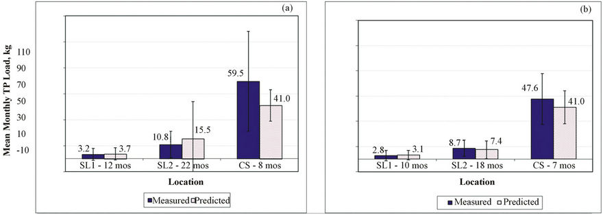
Figure 3. Measured and predicted mean monthly TP loads for SL1, SL2, and CS (a) with all data and (b) with exclusion of TP values for months with very large events. Also shown are the standard deviations as error bars.
lands. The proportions of organic P were higher than the mineral P for subareas draining the upstream agricultural lands and highways. The mean monthly predicted TP load of 15.5 kg for 22-month period was 43.2% higher than the measured (10.8 kg) (Figure 3(a)).
Data in Figure 3(b) shows the mean monthly TP load without the months with very large events in May and October 2008 and February and July of 2009. With the removal of these months in the analysis, the predicted mean monthly load of 7.4 kg for the 18-month was under-predicted by just 14.5% compared to the measured monthly mean of 8.7 kg. Overall, the TP predictions were deemed satisfactory given the limitations of the data, including some uncertainty for the flow and water quality both of which may impact predictions [53]. Other factors affecting predictions may be management practices and the model parameters as was done in a detailed comprehensive study by [15] in their study of assessment and management of reservoir water quality in Texas.
3.2.3. Cave Spring (CS) Outlet
The mean monthly predicted and measured total phosphorus (TP) for the months of January to August in 2009 at the cave spring (CS) outlet are presented in Figure 3(a). The model substantially underpredicted TP load in April (not shown). Due to the wide variability in measured concentration in April with the spring grab sampling data, the load estimated by a mass balance approach [7] that was input into the model was much smaller than the load calculated at the CS using measured concentrations and flows at various time intervals in the month [7]. Ground water flow contributing from an unknown area to the CS outlet resulted in 50% of the TP load [8]. The reason for such a high P in this groundwater is unknown whether it is a pollution or due to phosphate limestone, and is currently under investigation. This resulted in the mean monthly bias as high as 18.5 kg underprediction. For January to June, the measured concentrations in base flow (groundwater) as part of the total flow at the CS outlet [8] were not available, and estimated using a mass balance approach with the mean measured concentrations and total flow at SL7, CS, and baseflow, assumed as groundwater (GW) [7]. Accordingly, the mean monthly (for 8 months in 2009) predicted TP load was 41 kg compared to 59.5 kg of the measured load (Figure 3(a)) with a mean relative error of 31.1% underprediction. When the high value of April with wet conditions due to high lake levels was removed, the long-term mean predicted load of 41 kg for a 7-month period was underpredicted by just 6.6 kg compared to the measured data of 47.6 kg (Figure 3(b)). This was an underprediction of just 14.0%.
Some of these discrepancies between measured and predicted TP loads may also be attributed to sampling approaches. Reference [54] reported that accurately recording transient variations at karst springs requires more rigorous sampling strategies than traditional methods. Furthermore, a time proportional sampling had been used at the CS outlet rather than the flow-proportional sampling used at SL1 and SL2. Reference [55] reported the flow proportional sampling as the most accurate and sample intensive. Recently, [56] recommended a sampling frequency of 30 hours to achieve an uncertainty within 10% of the measured value for TP. Therefore, these calculated statistics for the long-term mean TP loadings were considered satisfactory for the limitations in length of the flow and sampling frequency of TP data, as well as the data for management practices draining the land at this cave spring (CS) outlet.
3.3. TP Prediction at Embayment (R-E)
The predicted flow-weighted monthly TP concentrations for the 34-month (January 2007 to October 2009) period were compared to the measured monthly data from SC014 in the embayment (Figure 4). The state standard of 0.06 mg/L for TP is also provided for comparison to examine the frequency and timing of violations for both the measured and SWAT predicted values. SWAT consistently overpredicted the measured TP values at SC014 for the measurement period, except in the last few months of 2009, when observed TP concentrations were as high as 0.6 mg/L and SWAT underpredicted the concentrations. Two of these high measurements occurred in the months of April and May 2009 (Figure 4) when lake levels were high, with possible suspended sediment influencing TP concentrations due to rising lake levels leading to perturbation of the bottom sediment. Also, visual observations confirmed that during May-June of 2009 an algal bloom occurred near SC014 and upstream of the SL2 outlet. The third high TP concentration on August 31, 2009 was observed after a large rain event which may have been influenced by either stormwater runoff, lake perturbation, or a combination of both. Another discrepancy for SWAT overprediction of measured data at this R-E embayment is possibly because the monthly sampling dates at SC014 seldom matched our sampling dates at the three locations used as input discharges to the R-E containing the SC014 modeled as a reservoir. Also monthly sampling at SC014 often occurred before the occurrence of large rainfall events for the month when the concentrations were low. For example, in the wettest month (October 2008) of the study period, the SC014 sample was taken on October 8, 2008, just prior to a very large rainfall event that started on October 9. Furthermore, there was another large rainfall event on October 24 [8,9,27]. Another overprediction occurred on July 21, 2009 (Figure 4) when sampling was conducted during a low flow period after a large rainfall event on July 16-17 as well as other relatively large storms earlier that month. Phosphorus attached to the sediment is generally washed off during the high runoff events [16,43]. But also, a dilution effect due to rainfall and runoff may have also caused the measured TP to be lower than that predicted by SWAT. Therefore, the prediction of flow-weighted TP concentration based on average for the whole month could be larger due to large runoff than the once in a month measured value during the low flow period.
The corresponding SWAT simulated monthly TP loads are compared in Figure 5 with those obtained by using
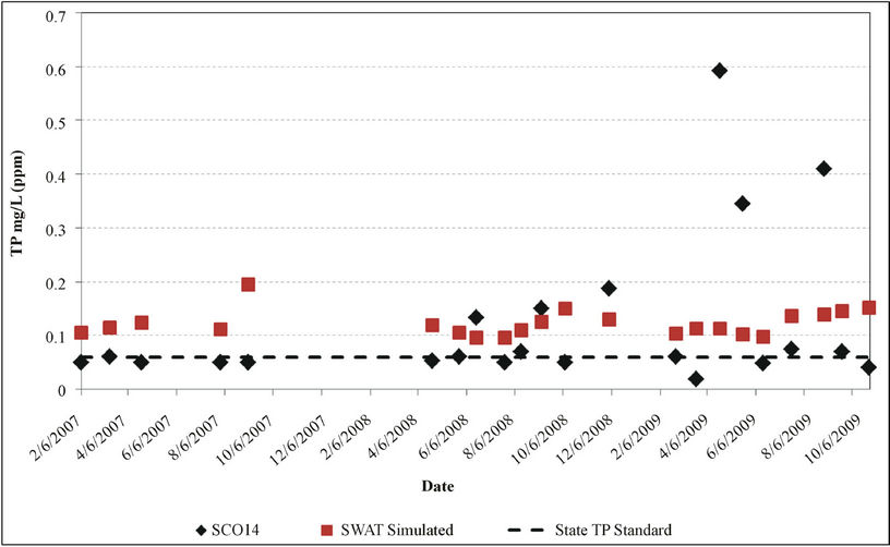
Figure 4. SWAT predicted TP concentrations compared with the measurements at SC014 in the R-E embayment for the 34 month (2007-2009) period. Broken line is allowable state standard of 0.06 mg/L.
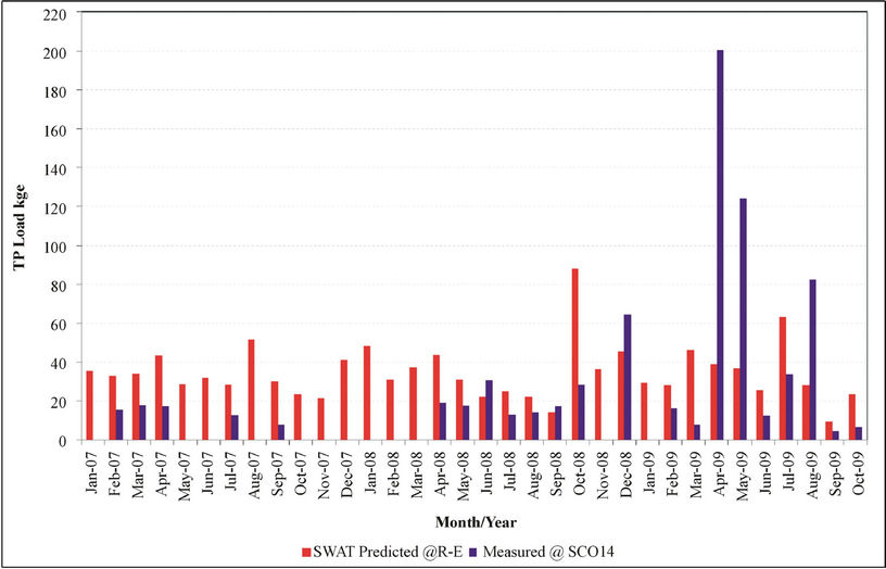
Figure 5. SWAT predicted TP loads compared with the estimated loads using the TP concentration measurements at SC014 in the R-E embayment for the 34 month (2007-2009) period. Estimated loads were not available for some months due to unavailability of measured concentration data.
the monthly measured TP concentrations (when available) with reservoir outflow estimate obtained by a water balance approach presented by [8]. Clearly, the measured monthly loads for the months (April and May of 2009) with very high (>0.34 mg·L−1) measured TP concentrations were substantially underpredicted by SWAT. Similarly, SWAT dramatically overpredicted the TP load in the wet month of October 2008 (Figure 5) during low lake levels first due to over-prediction of flow in that month [27] and secondly perhaps due to lower TP concentration measured just before the large event. The variability of estimated monthly TP loads was much higher (COV = 1.26) compared to only 0.48 of the COV for the SWAT predicted values, indicating a wider variability in monthly measured data. As a result, there was no correlation (R2 = −0.09) between the predicted and measured monthly TP loads (Figure 6(a)).
However, when months with very high measured TP values (April, May in 2009) and large discrepancies in flow measurements with overpredictions during low lake level (e.g. April and October in 2008) and underpredictions during higher lake levels (e.g. June 2008 and March and August in 2009) as reported by [27] were omitted in the analysis, the correlation substantially increased to adjusted R2 = 0.57 for a zero intercept (not significant at α = 0.05), although with a biased slope of 0.49 significant at p = 0.0005 (Figure 6(b)). These results indicate that the model may be able to predict the monthly TP loading, except for conditions with very low and high lake levels and very high TP levels, consistent with the findings by [16], and that such prediction may be double, on average, of the observed monthly TP loads calculated with one monthly TP value.
On an annual basis, clearly the predicted annual loads for 2007 and 2008 were much higher (nearly double or more) than the measured loads (not shown). The annual flow was under-predicted by about 9% in 2007 and overpredicted by about 40% in 2008 when the lake levels were low in this karst watershed [27]. So a reason for the overprediction of the TP load was attributed to the use of monthly (only once a month) measured TP concentrations stated earlier. However, the overprediction of TP load in 2008 may possibly due to overprediction of flows or once a month measurement of TP or both. Due to very high monthly measured values of TP concentration in the March, April, and May of 2009 with higher lake levels, the predicted TP load was 33% lower than the estimated, although the total flow was over-predicted by only about 2%. Conversely, the total predicted load of 761 kg for 22 months (from February 2007 to October 2009 only when the measured TP data was available; mean = 34.6 kg/mo) was only 13.3% overprediction compared to the estimated TP load of 672 kg (mean = 30.6 kg/mo) for the same period, indicating that the model’s prediction is acceptable on a longer term basis. These relative errors are similar or smaller than those obtained by [52] for phosphorus load predictions for calibration and validation periods using the SWAT model in the Wister Lake basin in Oklahoma, U.S.A.
Plots in Figure 7 show the comparison of SWAT simulated (A) monthly TP loads and (B) monthly cumulative TP loads from three major tributaries of SL1, SL2, and CS with the net loads (remaining load after all losses due to settling, uptake, and storage) simulated in the reservoir for 2007-2009 period. Reference [8] noted that despite high TP concentrations in flow from the subwatershed SL1, it contributed relatively little to the overall nutrient loading of the embayment due to relatively small flow. The simulated reservoir TP loads tend to follow the peaks of the total input from three tributaries in most of the wet months including August 2007, October 2008, and July 2009, while few small peaks were also dampened (Figure 6(a)). Clearly, the net monthly TP loads in the embayment were less than the combined inputs from
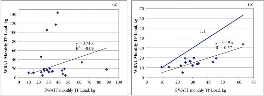
Figure 6. Regression of monthly measured or estimated with a water balance (WBAL) approach and SWAT predicted TP loads at the R-E embayment for (a) all the TP level measurement periods in 2007-2009 and (b) for the same period with removal of months with very high TP levels and/or large discrepancies in SWAT flow predictions as shown by [31].
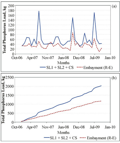
Figure 7. Simulated combined inputs of TP loadings from three subwatersheds (SL1, SL2, and CS): (a) Monthly loads, (b) Cumulative monthly loads compared to the net TP loadings in the embayment (R-E) for the 34-month (2007-2009) period.
the three tributaries in most of the months, as expected, indicating the loss of TP. The largest monthly losses as shown in Figure 7(a) were obtained for August 2007 (125 kg or 71%), July 2009 (118 kg or 63%), and October 2008 (62 kg or 41%). The mean monthly input was 59.6 kg compared to the net load in the reservoir of 34.6 kg yielding a loss of 25 kg or (58%), on average. The predicted total cumulative load from the three tributaries was 2028 kg compared to 1128 for the net TP load exported by the R-E embayment, indicating a loss of 42% TP load (850 kg) (Figure 7(b)).
The regression relationship of predicted monthly total TP input from SL1, SL2, and CS outlets to the net TP load in the embayment shown is significant with (R2 = 0.54, p < 0.00001), as expected. The relationship shows an intercept of 17.1 even when the input from the tributaries is zero, indicating possibly as a background TP level of 17.1 kg in the watershed embayment at SC014.
Simulation results indicated that the reservoir loading hydrodynamics in the R-E embayment led to a reduction in TP export and thus improvement in water quality delivered to Lake Marion. This reduction was also demonstrated by the measured data. The R-E may allow for particle settling processes that could contribute to reduced TP export, as the R-E residence time has been determined to vary between 4 to 9 weeks due to varying Lake Marion water levels [8]. Total phosphorus export was generally lower than the inputs, although the high inputs did result in a delayed peak export to Lake Marion. Both the data and simulation results for the 10-month measurement period (January-October 2009) showed greater variability in measured monthly TP concentrations than the estimated monthly outflows at the downstream embayment. This variability resulted in TP load inequality being greater than the flow inequality which may have implications in water quality management as was recently shown by [57].
3.4. Summary and Conclusions
A widely used watershed-scale distributed hydrologic model, SWAT2005 version, was applied to test its ability to predict monthly mean total phosphorus (TP) concentrations and loadings of a karst-affected watershed in the Upper Coastal Plain region of South Carolina, USA with a minimal calibration. Results of flow calibration and validation of the 1555 ha mixed land use watershed with its flooded embayment outlet draining to Lake Marion using the SWAT2005 have been recently published [27]. In this study, efforts were made to manually calibrate the model with limited monthly P loads measured at outlets of two tributaries (SL2 and CS) draining multiple subwatersheds, and an individual subwatershed (SL1). The SWAT mean monthly TP load predictions were within acceptable error limits at SL1 and SL2 only after removing months with high flows. Some of the discrepancies may be attributed to the use of default model parameters or literature based model input parameters for phosphorrus cycling and transport processes and not calibrating for the sediment yield due to lack of data. Other discrepancies may be attributed to the flow predictions in this complex karst watershed and to interaction with downstream lake water levels as argued by [27] and demonstrated by [8,9]. Potential measurement errors in the flow (particularly at the cave spring (CS) outlet) and sampling methods might also have contributed to model over-and underpredictions. Discrepancies were most apparent at the SL2 location with more suspected karst features [9,58] that also drains the most developed areas of the watershed, where high surface runoff and specifically TP loads can potentially occur. At the CS outlet, the simulated mean TP load was substantially biased by a large measured value in April 2009 and also possibly by some errors in estimated TP concentrations in sustained groundwater from a larger unknown subsurface area [8,9].
The observed discrepancies between the SWAT simulated results of TP loads and concentrations compared to the measured data at the flooded embayment R-E outlet receiving loadings from those three tributaries were attributed possibly to the limitations in measurements done only once a month generally before or after storm events. However, despite the influence of karst features and their interaction with lake water levels on flow and loadings from three input tributaries, SWAT’s 13% overprediction of long-term mean monthly TP load at this embayment was well within the acceptable limit. This indicates the potential capability of the SWAT application with its simplified hydrodynamic model for estimating mean monthly outflow as well as the TP load when the resources are limited for the additional use of complex models in an embayment where complete mixing can be assumed and loss is assumed primarily by settling rate. Simulation results showed that the 42% of the total incoming simulated TP load from all three tributaries embayment was lost in the embayment, indicating the potential of the SWAT model to be applied for assessments of TP loads from various source areas toward TMDL development for the CBC watershed.
Future studies should consider using the LiDAR-based finer DEMs for detecting karst features like depressions and sink holes in the CBC [59] and similar other watersheds which could be modeled more precisely using the most recent enhancements in SWAT [25,26]. Even with such modifications, the uncertainty in subsurface conduits may pose challenges in predicting groundwater contribution to streamflow [22,23] and pollutant loadings. Furthermore, a more detailed TP calibration of this watershed with field measured parameters on crop managements, fertilizer application rates/timings, and soil nutrient concentrations as shown by [60] should improve the predictions. Similarly, a longer term data for the tributaries (source areas, particularly at the groundwater (GW) portion of the discharge at the CS outlet) and frequent sampling in the embayment are also recommended to improve the predictions of the TP loadings from various source areas and also at the flooded R-E embayment outlet. Current planned research by SC DHEC to study the potential effects of limestone bedrock weathering versus anthropogenic sources on phosphorus loading in the CBC watershed could improve the model calibration and results.
4. Acknowledgements
This work was made possible by the support from South Carolina Department of Health and Environmental Control’s 319 Grant Agreement # EQ-7-514 (Project # 4OFY06) through a Forest Service collection agreement # 06- CO-11330135-122, which provided support to the Belle W. Baruch Institute of Coastal Ecology and Forest Science at Clemson University for conducting this study. The authors would like to acknowledge the contributions of Santee Cooper Biological and Analytical Laboratory for analyzing all water quality samples and SC DHEC staff for providing ample guidance on the project. Similarly, Liz Mihalik, former College of Charleston graduate student, Dr. Norm Levine, Associate Professor, College of Charleston, Town of Santee, SC State Park, Santee Golf National, Orangeburg County Soil Conservation District, SC Department of Transportation, US Army Corps of Engineers, Andy Harrison, Hydrotech, US Forest Service, Mathews Krasowski, David Joyner, former College of Charleston graduate student, and Weyerhaeuser Company are also acknowledged for their various levels of support and contribution during the project study phase. The authors are also thankful to Dr. Dan Tufford at University of South Carolina for providing constructive suggestions and comments in the manuscript.
REFERENCES
- E. J. B. Gaddis and A. Voinov, “Spatially Explicit Modeling of Land Use Specific Phosphorus Transport Pathways to Improve TMDL Load Estimates and Implement Planning,” Water Resources Management, Vol. 24, No. 8, 2010, pp. 1621-1644. doi:10.1007/s11269-009-9517-z
- B. Beltran, D. M. Amatya, M. A. Youssef, M. Jones, R. W. Skaggs, T. J. Callahan and J. E. Nettles, “Impacts of Fertilization Additions on Water Quality of a Drained Pine Plantation in North Carolina: A Worst Case Scenario,” Journal of Environmental Quality, Vol. 39, No. 1, 2010, pp. 293-303. doi:10.2134/jeq2008.0506
- G. F. Lee, “Evaluating Nitrogen and Phosphorus Control in Nutrient TMDLs,” Stormwater, 2002. http://www.stormh2o.com/forms/print-7447.aspx
- US EPA, “Factsheet: Introduction to Clean Water Act CWA Section 303 (d) Impaired Water Lists,” USEPA Office of Water, TMDL Program Results Analysis Fact Sheet, 17 July 2009. http://www.epa.gov/owow/tmdl/results/pdf/aug_7_introduction_to_clean.pdf
- SC Department of Health and Environmental Control (SCDHEC), “Watershed Water Quality Assessment— Santee River Basin,” Report No. 013-05, SCDHEC, Columbia, 2005.
- SC Department of Health and Environmental Control (SCDHEC), “State of South Carolina Integrated Report Part I: Listing of Impaired Waters,” 2008. http://www.scdhec.gov/environment/water/tmdl/docs/tmdl_08-303d.pdf
- D. M. Amatya, T. M. Williams, A. E. Edwards and D. R. Hitchcock, “Final Draft Report with Appendices on ‘Total Maximum Daily Load (TMDL) Development for Phosphorus: Chapel Branch Creek (SC014)’,” Submitted to SC Department of Health & Environmental Control, Bureau of Water, Division of Water Quality, Columbia, 2010.
- T. M. Williams, D. M. Amatya, D. R. Hitchcock and A. E. Edwards, “Streamflow and Nutrients from a Karst Watershed with a Downstream Embayment: Chapel Branch Creek,” Journal of Hydrologic Engineering, 2013, in press.
- A. E. Edwards, D. M. Amatya, T. M. Williams and D. R. Hitchcock, “Flow Characterization in the Santee Cave System in the Chapel Branch Creek Watershed, Upper Coastal Plain of South Carolina, USA,” Journal of Caves and Karst Studies, 2013, in press.
- D. M. Amatya, G. M. Cheschier, G. P. Fernandez, R. W. Skaggs and J. W. Gilliam, “DRAINWAT-Based Methods for Estimating Nitrogen Transport on Poorly Drained Watersheds,” Transactions of the ASAE, Vol. 47, No. 3, 2004, pp. 677-687.
- A. Gollamudi, C. A. Madramotoo and P. Enright, “Water Quality Modeling of Two Agricultural Fields in Southern Quebec Using SWAT,” Transactions of the ASABE, Vol. 50, No. 60, 2007, pp. 1973-1980.
- J. G. Arnold, R. Srinivasan, R. S. Muttiah and J. R. Williams, “Large Area Hydrological Modeling and Assessment. Part I: Model Development,” Journal of the American Water Resources Association, Vol. 34, No. 1, 1998, pp. 73-89. doi:10.1111/j.1752-1688.1998.tb05961.x
- D. L. Tufford, H. N. McKellar and J. R. Hussey. “InStream Nonpoint Source Nutrient Prediction with LandUse Proximity and Seasonality,” Journal of Environmental Quality, Vol. 27, No. 1, 1998, pp. 100-111. doi:10.2134/jeq1998.00472425002700010015x
- D. L. Tufford and H. N. McKellar, “Spatial and Temporal Hydrodynamic and Water Quality Models of a Large Reservoir on the South Carolina (USA) Coastal Plain,” Ecological Modelling, Vol. 114, No. 2-3, 1999, pp. 137-173. doi:10.1016/S0304-3800(98)00122-7
- B. Narasimhan, R. Srinivasan, S. Bednarz, M. Ernst and P. M. Allen, “A Comprehensive Modeling Approach for Reservoir Water Quality Assessment and Management Due to Point and Nonpoint Source Pollution,” Transactions of the ASABE, Vol. 53, No. 5, 2010, pp. 1605-1617.
- D. K. Borah and M. Bera. “Watershed-Scale Hydrologic and Nonpoint-Source Pollution Models; Review of Applications,” Transactions of the ASAE, Vol. 47, No. 3, 2004, pp. 789-803.
- P. B. Parajuli, N. O. Nelson, L. D. Frees and K. R. Mankin, “Comparison of AnnAGNPS and SWAT Model Simulation Results in USDA-CEAP Agricultural Watersheds in South-Central Kansas,” Hydrological Processes, Vol. 23, No. 5, 2009, 748-763. doi:10.1002/hyp.7174
- M. K. Jha, P. W. Gassman and J. G. Arnold, “Water Quality Modeling for the Racoon River Watershed Using SWAT,” Transactions of the ASABE, Vol. 50, No. 2, 2007, pp. 479-493.
- C. Santhi, J. G. Arnold, J. R. Williams, W. A. Dugas, R. Srinivasan and L. M. Hauck. “Validation of the SWAT Model on a Large River Basin with Point and Nonpoint Sources,” Journal of the American Water Resources Association, Vol. 37, No. 5, 2001, pp. 1169-1188. doi:10.1111/j.1752-1688.2001.tb03630.x
- G. K. Felton, “Hydrologic Responses of a Karst Watershed,” Transactions of the ASAE, Vol. 37, No. 1, 1994, pp. 143-150.
- C. A. Spruill, S. R. Workman and J. L. Taraba, “Simulation of Daily and Monthly Stream Discharge from Small Watersheds Using the SWAT Model,” Transactions of the ASAE, Vol. 43, No. 6, 2000, pp. 1431-1439.
- H. Jourde, A. Roesch, V. Guinot and V. Bailly-Comte, “Dynamics and Contribution of Karst Groundwater to Surface Flow during Mediterranean Flood,” Environmental Geology, Vol. 51, No. 5, 2007, pp. 725-730. doi:10.1007/s00254-006-0386-y
- F. Salerno and G. Tartari, “A Coupled Approach of Surface Hydrological Modeling and Wavelet Analysis for Understanding the Base Flow Component of River Discharge in Karst Environments,” Journal of Hydrology, Vol. 376, No. 1-2, 2009, pp. 295-306. doi:10.1016/j.jhydrol.2009.07.042
- K. L. White, I. Chaubey, B. E. Haggard and M. D. Matlock, “Comparison of Two Methods for Modeling Monthly TP Yield from a Watershed,” ASAE/CSAE Meeting Paper # 04-2162, ASAE, St. Joseph, 2004.
- C. Baffaut and V. W. Benson, “Modeling the Flow and Pollutant Transport in a Karst Watershed with SWAT,” Transactions of the ASABE, Vol. 52, No. 2, 2009, pp. 469- 479.
- G. A. Yachtao, “Modification of the SWAT Model to Simulate Hydrologic Processes in a Karst Influenced Watershed,” MS Thesis, Virginia-Tech, Department of Biosystems Engineering, Blacksburg, 2009.
- D. M. Amatya, M. K. Jha, A. E. Edwards, T. M. Williams and D. R. Hitchcock, “SWAT-Based Streamflow and Embayment Modeling of a Karst Affected Chapel Branch Watershed, SC,” Transactions of the ASABE, Vol. 54, No. 4, 2011, pp. 1311-1323.
- Ambrose, R. B., T. A. Woll, J. L. Martin. “WASP5.x, a Hydrodynamic and Water Quality Model: Model Theory, User’s Manual and Programmers’ Guide,” US Environmental Protection Agency (EPA), Athens, 1991.
- B. L. Hockensmith, “Potentiometric Surface of the Floridan Aquifer and Tertiary Sand Aquifer in South Carolina,” SC Department of Natural Resources Water Resources Report 48, 2004.
- P. J. Moore, J. B. Martin and E. J. Screaton, “Geochemical and Statistical Evidence of Recharge, Mixing, and Controls on Spring Discharge in an Eogenetic Karst Aquifer,” Journal of Hydrology, Vol. 376, No. 3, 2009, pp. 443-455. doi:10.1016/j.jhydrol.2009.07.052
- ERC, “Drainage Analysis of SCDHEC DAM #D-3746 (Lower Santee Shores Dam) Santee,” Engineering Resources Corporation, 1999, 53 p.
- E. N. Mihalik, N. S. Levine and D. M. Amatya, “Rainfall-Runoff Modeling of the Chapel Branch Creek Watershed Using GIS-Based Rational and SCS-CN Methods,” Paper No. 083971, ASABE, St. Joseph, 2008.
- E. N. Mihalik, “Watershed Characterization and Runoff Modeling of the Chapel Branch Creek, Orangeburg County, South Carolina,” MS Thesis, College of Charleston, SC Department of Environment and Geosciences, Charleston, 2007, 127 p.
- L. Turc, “Evaluation de Besoins en eau D’irrigation, ET Potentielle,” Annals of Agronomiques, Vol. 12, No. 1, 1961, pp. 13-49.
- D. M. Amatya, R. W. Skaggs and J. D. Gregory, “Comparison of Methods for Estimating REF-ET,” Journal of Irrigation and Drainage Engineering, Vol. 121, No. 6, 1995, pp. 427-435. doi:10.1061/(ASCE)0733-9437(1995)121:6(427)
- A. D. Eaton, L. S. Clesceri, E. W. Rice and A. E. Greenberg, “Standard Methods for Examination of Water and Wastewater,” 21st Edition, American Public Health Association (APHA), American Water Works Association, and Water Pollution Control Federation, Washington DC, 2005.
- C. Santhi, J. G. Arnold, J. R. Williams, W. A. Dugas and L. M. Hauck, “Application of a Watershed Model to Evaluate Management Effects on Point and Nonpoint Source Pollution,” Transactions of the ASAE, Vol. 44, No. 6, 2002, pp. 1559-1570.
- P. W. Gassman, M. R. Reyes, C. H. Green and J. G. Arnold, “The Soil and Water Assessment Tool: Historical Development, Applications, and Future Research Directions,” Transactions of the ASABE, Vol. 50, No. 4, 2007, pp. 1211-1250.
- K. R. Douglas-Mankin, R. Srinivasan and J. G. Arnold, “Soil and Water Assessment Tool (SWAT) Model,” Current Developments and Applications, Vol. 53, No. 5, 2010, pp. 1423-1431.
- C. Santhi, J. R. Williams, W. A. Dugas, J. G. Arnold, R. Srinivasan and L. M. Hauck, “Water Quality Modeling of Bosque River Watershed to Support TMDL Analysis,” TMDL Environmental Regulations: Proceedings of the Fort Worth, 11-13 March 2002, pp. 33-43.
- M. K. Jha, C. F. Wolter, P. W. Gassman and K. E. Schilling, “Assessment of TMDL Implementation Strategies for Nitrate Impairment of the Raccoon River, Iowa,” Journal of Environmental Quality, Vol. 39, No. 4, 2010, pp. 1317-1327. doi:10.2134/jeq2009.0392
- D. K. Borah, G. Yagow, A. Saleh, P. L. Barnes, W. Rosenthal, E. C. Krug and L. M. Hauck, “Sediment and Nutrient Modeling for TMDL Development and Implementation,” Transactions of the ASAE, Vol. 49, No. 4, 2006, pp. 967-986.
- W. G. Knisel, “CREAMS: A Field-Scale Model for Chemicals, Runoff and Erosion from Agricultural Management Systems,” USDA Conservation Research Report, Vol. 26, No. 1, 1980, pp. 36-64.
- D. K. Borah and M. Bera, “Watershed-Scale Hydrologic and Nonpoint-Source Pollution Models; Review of Applications,” Transactions of the ASAE, Vol. 47, No. 3, 2004, pp. 789-803.
- T. S. Ramanarayanan, R. Srinivasan and J. G. Arnold, “Modeling Wister Lake Watershed Using a GIS_Linked Basin Scale Hydrologic/Water Quality Model,” 3rd International Conference Workshop on Integrating Geographic Information Systems and Environmental Modeling, National Center for Geographic Information and Analysis, Sante Fe, 21-25 January 1996.
- K. L. White, I. Chaubey, B. E. Haggard and M. D. Matlock, “Comparison of Two Methods for Modeling Monthly TP Yield from a Watershed,” Proceedings of American Society of Agricultural Engineers, Ottawa, 1-4 August 2004.
- S. L. Neitsch, J. G. Arnold, J. R. Kiniry, J. R. Williams and K. W. King, “Soil and Water Assessment Tool Theoretical Documentation, Version. 2000,” USDA-ARS Blackland Research Center, Temple, 2002.
- T. M. Williams, D. M. Amatya, D. R. Hitchcock, N. Levine and E. N. Mihalik, “Chapel Branch Creek TMDL Development: Integrating TMDL Development with Implementation,” 2007 ASABE Annual International Meeting, Minneapolis, 17-20 June 2007, 13 p.
- S. L. Neitsch, J. G. Arnold, J. R. Kiniry, R. Srinivasan and J. R. Williams, “Soil and Water Assessment Tool SWAT Input/Output File Documentation, Versions. 2003,” USDAARS Blackland Research Center, Temple, 2004.
- J. H. Gakstatter, M. O. Allum, S. E. Dominguez and M. R. Crouse, “A Survey of Phosphorus and Nitrogen Levels in Treated Municipal Wastewater,” Journal Water Pollution Control Federation, Vol. 50, No. 4, 1978, pp. 718-722.
- L. Chiang, I. Chaubey, M. W. Gitau and J. G. Arnold, “Differentiating Impacts of Land Use Changes from Pasture Management in a CEAP Watershed Using the SWAT Model,” Transactions on ASABE, Vol. 53, No. 5, 2010, pp. 1569-1584.
- P. R. Busteed, D. E. Storm, M. J. White and S. H. Stoodley, “Usin GSWAT to Target Critical Source Sediment and Phosphorus Areas in the Wister Lake Basin,” American Journal of Environmental Sciences, Vol. 5, No. 2, 2009, pp. 156-613. doi:10.3844/ajessp.2009.156.163
- R. D. Harmel, R. J. Cooper, R. M. Slade, R. L. Haney and J. G. Arnold, “Cumulative Uncertainty in Measured Streamflow and Water Quality Data for Small Watersheds,” Transactions of the ASABE, Vol. 49, No. 3, 2006, pp. 689-701.
- M. Ryan and J. Meiman, “An Examination of Short-Term Variations in Water Quality at a Karst Spring in Kentucky,” Ground Water, Vol. 34, No. 1, 1996, pp. 23-30. doi:10.1111/j.1745-6584.1996.tb01861.x
- P. S. Miller, R. H. Mohtar and B. A. Engel, “Water Quality Monitoring Strategies and Their Effects on Mass Load Calculation,” Transactions of the ASABE, Vol. 50, No. 3, 2007, pp. 817-829.
- F. Birgand, T. W. Appelboom, G. M. Chescheir and R. W. Skaggs, “Estimating Nitrogen, Phosphorus and Carbon Fluxes in Forested and Mixed-Use Watersheds of the Lower Coastal Plain of North Carolina: Uncertainties Associated with Infrequent Sampling,” Transactions of the ASABE, Vol. 54, No. 6, 2011, pp. 2099-2110.
- J. W. Jawitz and J. Mitchell, “Temporal Inequality in Catchment Discharge and Solute Export,” Water Resources Research, Vol. 47, No. 10, 2011, Article ID: W00J14. doi:10.1029/2010WR010197
- A. E. Edwards and D. M. Amatya, “Photo Essay: Recent Sinkhole Collapse,” South Carolina Geology Journal, Vol. 47, No. 1, 2010, pp. 17-18.
- A. E. Edwards, D. M. Amatya, T. M. Williams and D. R. Hitchcock, “A Water Quality Study Recommends Protection of a Karst Watershed in the Upper Coastal Plain of South Carolina,” National Speleological Society News, Vol. 69, No. 4, 2011, pp. 17-19.
- [61] K. R. Douglas-Mankin, D. Maski, K. A. Janssen, P. Tuppad and G. M. Pierzynski, “Modeling Nutrient Yields from Combined In-Field Crop Practices Using SWAT,” Transactions of the ASABE, Vol. 53, No. 5, 2010, pp. 1557-1568.