Received 30 November 2015; accepted 27 March 2016; published 30 March 2016

ABSTRACT

Assuming a flat universe expanding under a constant pressure and combining the first and the second Friedmann equations, a new equation, describing the evolution of the scale factor, is derived. The equation is a general kinematic equation. It includes all the ingredients composing the universe. An exact closed form solution for this equation is presented. The solution shows remarkable agreement with available observational data for redshifts from a low of z = 0.0152 to as high as z = 8.68. As such, this solution provides an alternative way of describing the expansion of space without involving the controversial dark energy.

Keywords:

Cosmological Constant, Distances and Redshifts, Expanding Universe, Friedmann Equations

1. Introduction

The evolution of the universe has already been investigated through the first Friedmann equation. As discussed by Carrol [1] , the first Friedmann equation is used because it only involves the first derivative of the scale factor. However, the resulting models such as ΛCDM-based models are in terms of limited numbers of parameters representing the ingredients of the universe. Two analytical solutions with restrictive assumptions are already available [2] [3] , which will be presented in Section three. There exists no general analytical solution for the Friedmann equations. Here, through combining the first and the second Friedmann equations, a general equation is formulated. Assuming a flat universe, an exact closed form solution for this general equation is obtained. This solution is remarkably consistent with the observational data over a wide range of measured redshifts from a low of z = 0.0152 to the highest recently measured value of z = 8.68.

Except for the flatness assumption, the analytical solution is completely general. It includes all the ingredients forming the universe. The ΛCDM-based models only consider specific combinations of limited numbers of ingredients. Also the value of the cosmological density parameter is analytically estimated to be. This is essentially identical to the value estimated in 2014 by the Plank Collaboration [4] , based on combined data from “Plank + WP + high L + BAO”. It is also shown that the contribution of the cosmological constant is to cancel the pressure term in the Friedmann acceleration equation. As a consequence, the expansion equation turns out to be a kinematic equation in terms of the scale factor and its rates of change.

In the next section we develop the new general equation and derive an analytical estimate of the cosmological density parameter. The new analytical solution together with the two existing analytical solutions is presented in Section 3. Comparison of the new analytical solution with the analytical solution involving matter and lamda is presented in Section 4.1. Comparisons of the new analytical solution with the ΛCDM-based models are presented in Section 4.2. In Section 5, the efficacy of the new analytical solution is shown through comparisons with two ΛCDM-based solutions and through comparisons with three sets of observational data.

2. The New General Equation

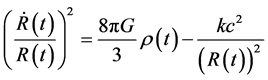
The first Friedmann equation, including the curvature, k, and the cosmological constant, Λ, is

(1)

Alternatively, including the cosmological term in the total density, the above equation can be represented by

(2)

where now the density, , is defined by

(3)

where represents the mass density; represents the energy density; represents the radiation energy density and is the intrinsic vacuum energy density, which is defined by

(4)

The curvature can be represented by

(5)

where represents the present time and is the scale factor. The Friedmann acceleration equation is given by

(6)

Substitutions for from Equation (2) and for k from Equation (5) back into the above equation yield

(7)

For the present time, , the scale factor,. Thus the above equation yields

(8)

To evaluate Λ from Equation (8), we need to evaluate first. The value of at the present time is given by

(9)

To evaluate the present time values of and, consider the conservation of energy or the alternative form of the first Friedman equation

(10)

where is an equivalent mass. It represents the total mass-energy of the universe including the total mass of all forms of ordinary and non-ordinary masses as well as the total equivalent mass of all forms of energies; including the effect of the cosmological constant. Because of the conservation of the total mass-energy of the un

iverse, has to be a constant. But. Therefore

(11)

Because at all points the expansion is taking place in all directions, to evaluate the rate of increase of space between any two galaxies, must be replaced by. Thus

(12)

Correcting the velocity in the above relation for the effect of time dilation yields

(13)

where c represents the speed of light. The value of has been analytically determined [5] to be

(14)

Therefore the corrected expansion velocity at the present time is given by

(15)

Also the present time value of the expansion acceleration, according to Equations (13) and (14), is given by

(16)

Substitutions for from Equation (9), for the corrected velocity from Equation (15), and for from Equation (16) back into Equation (8) yields

(17)

Solving the above relation for Λ yields

(18)

Therefore the cosmological density parameter can be represented by

(19)

Now substitution for Λ from Equation (18) back into Equation (7) yields the Friedmann acceleration equation as

(20)

In the next section, assuming a flat universe expanding under the constant pressure, we present an exact closed form solution for the above equation. Before getting to the next section, we will evaluate the value of the cosmological density parameter. The pressure, , in Equation (19) has been given by [5] the following relation

(21)

where

(22)

and

(23)

Assuming a flat universe, i.e., , substitutions of the above values into Equation (19) yield the cosmological density parameter as

(24)

This value of the energy density parameter is essentially identical to the value estimated in 2014 by the Plank Collaboration [4] , based on data from “Plank + WP + high L + BAO”. This remarkable agreement provides further evidence supporting the description of the pressure as given by Equation (21).

3. The New Analytical Solution for the Friedmann Equations

Already there exist two analytical solutions for the Friedmann equations. One is for the case of a flat universe containing only matter, , where the analytical solution is, and the other is for the case of a flat universe containing matter and lambda [2] [3] . The analytical solution for the second case is given as

(25)

where, is the scale factor and. The new analytical solution considers a flat universe containing all the ingredients including matter, energy, radiation, etc. Considering Equation (20), it is seen that as the time flows from the initiation of expansion to the present time, , the coefficient of the curvature term, k, reduces. Thus as time flows, the universe tends toward becoming flatter. Therefore, according to Equation (20), by the present time, , the universe has become completely flat. Assuming a flat universe eliminates the effects of curvature and simplifies the Friedmann acceleration equation to the following form

(26)

Assuming the pressure to be constant implies that in the above equation the term. Since represents the contribution of the cosmological constant, being zero is consistent with the vacuum

pressure being equal to the negative of the vacuum density as discussed by Carroll [6] . Thus the Friedmann acceleration equation is further simplified to the following form:

(27)

It is clear that the above equation satisfies the present time boundary conditions as given in Equations (9), (15) and (16). To non-dimensionalize the above equation, let and. Substitutions in the above equation yield

(28)

where now dot denotes differentiation with respect to, and represents the scale factor. The present time boundary conditions on the above equation, as derived from Equations (9) and (15), are and. The exact solution of the above nonlinear differential equation with the specified boundary conditions is

(29)

The beauty of the above analytical solution is the fact that it does not involve the fractional components forming the mix of the universe. Using the Mathematica code [7] , a plot of the scale factor as given by the above equation together with its first and second derivatives is presented in Figure 1.

As seen from the above figure, at the present time, , the scale factor, , and its rates of change are, , and. Based on observational data [8] - [10] , it has been concluded that the expansion initially decelerates but then continues to grow with an accelerating rate.

Considering Equation (18), it is clear that in Equation (20), the pressure represents the contribution of the cosmological constant. It is this pressure, , that cancels the constant pressure, P, allowing the Friedmann acceleration equation to be simplified to the form given by Equation (28).

In the following subsections the analytical solution given by Equation (29) is compared with the analytical solution for a universe containing only matter and lambda as given by Equation (25). It is also compared with other models based on ΛCDM parameterizations.

4. Comparison of Analytical Solutions

In order to compare the analytical solution given by Equation (29) with the one given by Equation (25), we need to first decide on the value of for substitution in Equation (25). We will use the analytically predicted value as given by Equation (24), i.e.,. The value of the constant C in Equation (25) is calculated by equating the present time value of the scale factor to unity. In this way, the value of C is determined to be. A plot of scale factors from Equations (25) and (29) is presented in Figure 2.

The time in Figure 2 represents the present time. For the new analytical solution, shown as a solid line in this figure, the zero time of the scale factor occurs at the time. Equation (29) describes the evolution of the scale factor for a flat universe including all its ingredients. The scale factor calculated from Equation (25), shown as a dashed line, is for a universe composed of matter and Λ only. Its zero time occurs at. The difference between these two analytical solutions is due to the fact that one of them includes all the ingredients of the universe and the other one considers a universe composed of a specified mix of only two ingredients, matter and Λ.

4.1. Comparisons of the New Solution with ΛCDM-Based Models

The ΛCDM-based models characterize the universe with a limited number of energy density parameters as fractions of constituent ingredients. The values of these fractions are estimated through finding the optimum fit to the observationally measured data. The results are presented in terms of distance modulus versus redshift. Here, a comparison of the variation of scale factors versus redshift will be carried out first. The relation between the scale factor and the redshift, z, is defined by

(30)

Thus

(31)

To express the scale factor given by Equation (29) in terms of redshift, substitution for the scale factor, a, from Equation (29) back into Equation (31) yields the relation between the red shift, z, and the time as

(32)

Using the above equation, the variation of time versus the redshift is presented in Figure 3.

In Figure 3 the present time, , corresponds to the redshift,. Consistent with this, for comparison with observational data, a transformation is made such that would correspond to the present time,. To this end the values of from Equation (29) and the values of the redshifts z from Equation (32)

are tabulated for values of varying from zero to one. Next the tabulated values of are plotted

versus the tabulated values of the redshift, z, in Figure 4. Through this process, corresponds to the present time,.

For ΛCDM-based models, considering Equation (30), and rewriting Friedmann Equation (2) in terms of fractions of constituent densities, for a universe containing mass, energy, radiation and curvature, one obtains the in terms of the redshift as

(33)

Using the above equation, the values of are plotted versus z in Figure 4 for two sets of ΛCDM-based parameters, estimated by the Plank Collaboration [4] , as presented in Table 1. As seen from Figure 4, the ΛCDM-based curves are consistent with the analytical curve. But they are not identical to the analytical curve. There are two reasons for not being identical. The first reason is the differences in the fractions of ingredients included in the models. The second reason is the fact that the initial times for the scale factors of the - based models are not defined.

In the next subsection the analytical curve and the curves based on ΛCDM parameterization are compared with the observational data.

4.2. Comparison of the New Solution with Observational Data

In this part the curve of the analytical scale factor given by Equation (29), transformed through Equation (32), is compared with the curves based on ΛCDM, as given by Equation (33), for the two different sets of ingredients presented in Table 1. To check how well these curves represent the reality, the following three sets of observational data will be used:

1) A set of 557 SNe data with redshifts from a low of to a maximum of, as reported in 2010 in the Union2 Compilation [11] ;

2) A set of 394 extragalactic distances to 349 galaxies at cosmological redshifts significantly higher than the Union2 Compilation with redshifts from a low of to a maximum of, as reported in 2008 by Mador and Steer [12] ;

3) A set of data for a quasar and the three most distant recently confirmed galaxies, as presented in Table 2.

To compare with the aforementioned observational data, the scale factors have to be presented in terms of distance modulus and redshift. The SNe and the Union2 data are already available in terms of distance modulus and redshift. The data for the galaxies and for the quasar are listed in Table 2, and, for the new analytical solution, the data for the scale factors in terms of distance modulus and redshift are represented through the following relation

(34)

where represents distance modulus; a represents the scale factor; is in megaparsecs and the factor represents the effects of observational data such as source luminosity, and data processing correc-

tions including the instrument corrections and the K-correction. These are well known corrections and they are

considered in various ways [17] - [20] . We evaluate the factor through matching of the analytical curve

with the first set of the observational data. Then we check the validity of its value through comparisons with the

second and third sets of observational data as well as with the ΛCDM-based curves. To evaluate, using

the analytical curve, we only need to have the value for the Hubble constant. The recent estimated values of the

Hubble constant based on observational data are: (the Seven-Year Wilkinson Microwave Anisotropy Probe [21] , 2011),; (the Planck Collaboration [4] , 2014),; (the Nine-Year Wilkinson Microwave Anisotropy Probe [22] , 2013),; and (the Megamaser Cosmology Project IV, [23] , 2013),. The average of these four values is. But most recently (Mostaghel [5] , 2015), the value of the Hubble constant is analytically estimated to be

(35)

Because this value is remarkably consistent with the observationally estimated values, we will use this value and substitute it together with the values of, as obtained through Equations (29) and (32), into Equation (34). Through matching the curve of Equation (34) with the first set of observational data presented in Figure 5, the factor is found to be given by

(36)

As can be seen from Figure 5, with this the analytically derived scale factor fits the first set of observational data remarkably well. Substitution for from the above equation back into Equation (35) yields the distance modulus as

(37)

where, c is in, and is in. The above relation directly gives the distance modulus in terms of the scale factor and the redshift.

Now, to check the validity of the factor, we include the second and the third sets of observational data. Equation (37) will be used to compare the analytical solution with the ΛCDM-based models and the observational data. The parameters for the ΛCDM curves are given in Table 1. For the analytical solution, as mentioned above, we use. The three sets of observational data, the analytical curve based

on Equations (29) and (32), and the two ΛCDM curves based on Equation (33), are presented in Figures 6-9. As seen from these figures, in all cases, the analytical curve is remarkably consistent with the observational data as well as with the ΛCDM-based curves. The log-linear plots and the linear plots show how well the curves represent the observational data at the low and high values of the redshifts respectively.

The excellent match of the analytical curve and the ΛCDM curves with the second and the third set of the observational data validates Equation (36) representing the factor. It also confirms the analytically eva-

luated value for the Hubble constant as given in Equation (35). It should be noted that, except for the flatness assumption, the analytical solution is completely general. It includes all the ingredients forming the universe. The ΛCDM-based solutions only consider specific combinations of limited numbers of ingredients.

5. Summary and Remarks

The value of the energy density parameter was analytically estimated to be. This value is essentially identical to the estimated value based on the observational data. This fact and the remarkable consis-

tency of the analytical solution with the observational data, as well as with the -based models, provide the necessary confidence in the fidelity of the analytical solution in the representation of reality.

The pressure is cancelled from the Friedmann acceleration equation through the contribution of the cosmological constant. As the result, Equation (28) may be interpreted as a kinematic equation. Its solution, Equation

(29) describes the evolution of the expansion of space. As such, this equation provides an alternative way of describing the expansion of space without involving the controversial dark energy.

Cite this paper

Naser Mostaghel, (2016) A New Solution for the Friedmann Equations. International Journal of Astronomy and Astrophysics,06,122-134. doi: 10.4236/ijaa.2016.61010

References

- 1. Carroll, S.M. (2013) Why Does Dark Energy Make the Universe Accelerate? Posted on 16 November.
http://www.preposterousuniverse.com/blog/2013/11/16/ - 2. Christiansen, J.L. and Siver, A. (2012) Computing Accurate Age and Distance Factors in Cosmology. arXiv: 1204. 0039v1 [astro-ph.CO], 30 March.
- 3. Ullrich, P. (2007) Exact and Perturbed Friedmann-Lemaitre Cosmologies. University of Waterloo, Ontario.
http://www-personal.umich.edu/~paullric/Ullrich-MastersThesis.pdf - 4. Ade, P.A.R., et al., Plank Collaboration (2014) Plank 2013 Results. XVI. Cosmological Parameters. arXiv: 1303. 5076v3 [astro-ph.CO], 20 March 2014.
- 5. Mostaghel, N. (2015) An Analytical Estimate of the Hubble Constant. American Journal of Astronomy and Astrophysics, 3, 44-49.
http://dx.doi.org/10.11648/j.ajaa.20150303.13 - 6. Carroll, S.M., Press, W.H. and Turner, E.L. (1992) The Cosmological Constant. Annual Review of Astronomy and Astrophysics, 30, 499-542.
http://www.nr.com/whp/CosmoConstAnnRev.pdf - 7. Wolfram Mathematica (2011) Version: 8.01.0.
- 8. Riess, A.G. (2012) Nobel Lecture: My Path to the Accelerating Universe. Reviews of Modern Physics, 84, 1165-1175.
http://dx.doi.org/10.1103/RevModPhys.84.1165 - 9. Schmidt, B.P. (2012) Nobel Lecture: Accelerating Expansion of the Universe through Observation of Distant Supernovae. Reviews of Modern Physics, 84, 1151-1163.
http://dx.doi.org/10.1103/RevModPhys.84.1151 - 10. Perlmutter, S. (2012) Nobel Lecture: Measuring the Acceleration of the Cosmic Expansion Using Supernovae. Review of Modern Physics, 84, 1127-1149.
http://dx.doi.org/10.1103/RevModPhys.84.1127 - 11. Amanullah, R., Lidman, C., Rubin, D., Aldering, G., Astier, P., Barbary, K., et al. (2010) Spectra and Hubble Space Telescope Light Curves of Six Types Ia Supernovae at 0.511< z < 1.12 and the Union2 Compilation. The Astrophysical Journal, 716, 712-738.
http://supernova.lbl.gov/Union/figur...n2_mu_vs_z.txt
http://dx.doi.org/10.1088/0004-637X/716/1/712 - 12. Mador, B.F. and Steer, I.P. (2008) NASA/IPAC Extragalactic Database Master List of Galaxy Distances. NED-4D.
http://ned.ipac.caltech.edu/level5/NED4D/ - 13. Zitrin, A., Labbe, I., Belli, S., Bouwens, R., Ellis, R.S., Roberts-Borsani, G., Stark, D.P., Oesch, P.A. and Smit, R. (2015) Lyman-Alpha Emission from a Luminous z = 8.68 Galaxy: Implications for Galaxies as Tracers of Cosmic Reionization. The Astrophysical Journal Letters, 810, L12.
https://en.wikipedia.org/wiki/List_of_the_most_distant_astronomical_objects>http://dx.doi.org/10.1088/2041-8205/810/1/L12
https://en.wikipedia.org/wiki/List_of_the_most_distant_astronomical_objects - 14. Oesch, P.A., Van Dokkum, P.G., Illingworth, G.D., Bouwens, R.J., Momcheva, I., Holden, B., Roberts-Borsani, G.W., Smit, R., Franx, M., Labbé, I., González, V. and Magee, D. (2015) A Spectroscopic Redshift Measurement for a Luminous Lyman Break Galaxy at z = 7.730 Using Keck/MOSFIRE. The Astrophysical Journal Letters, 804, L30.
http://dx.doi.org/10.1088/2041-8205/804/2/L30 - 15. Finkelstein, S.L., Papovich, C., Dickinson, M., Song, M., Tilvi, V., Koekemoer, A.M., et al. (2013) A Galaxy Rapidly Forming Stars 700 Million Years after the Big Bang at Redshift 7.51. Nature, 502, 524-527.
http://dx.doi.org/10.1038/nature12657 - 16. Matson, J. (2011) Brilliant, but Distant: Most Far-Flung Known Quasar Offers Glimpse into Early Universe. Scientific American, 29 June 2011.
http://eso.org/public/news/eso1122/ - 17. Peebles, P.J.E. (1993) Principles of Physical Cosmology. Princeton University Press, Princeton.
- 18. Peacock, J.A. (1999) Cosmological Physics. Cambridge University Press, Cambridge.
- 19. Hogg, D.W., Baldry, I.K., Blanton, M.R. and Eisenstein, D.J. (2002) The K Correction. arXiv:astro-ph/0210394v1.
- 20. Saunders, C., Aldering, G., Antilogus, P., Aragon, C., Bailey, S., Baltay, C., et al. (2014) Type IA Supernova Distance Modulus Bias and Dispersion from K-Correction Errors: A Direct Measurement Using Lightcurve Fits to Observed Spectral Time Series. The Astrophysical Journal, 800, 57.
http://dx.doi.org/10.1088/0004-637X/800/1/57 - 21. Larson, D., Dunkley, J., Hinshaw, G., Komatsu, E., Nolta, M.R., Bennett, C.L., et al. (2011) Seven-Year Wilkinson Microwave Anisotropy Probe (WMAP) Observations: Sky Maps, Systematic Errors, and Basic Results. Astrophysical Journal Supplement Series, 192, 16.
http://dx.doi.org/10.1088/0067-0049/192/2/16 - 22. Bennett, C.L., Larson, D., Weiland, J.L., Jarosik, N., Hinshaw, G., Odegard, N., et al. (2013) Nine-Year Wilkinson Microwave Anisotropy Probe (WMAP) Observations: Maps and Results. Astrophysical Journal Supplement Series, 208, 20.
http://dx.doi.org/10.1088/0067-0049/208/2/20 - 23. Reid, M.J., Braatz, J.A., Condon, J.J., Lo, K.Y., Kuo, C.Y., Impellizzeri, C.M.V. and Henkel, C. (2013) The Megamaser Cosmology Project IV. A Direct Measurement of the Hubble Constant from UGC 3789. Astrophysical Journal, 767, 154.
http://dx.doi.org/10.1088/0004-637x/767/2/154