A 3-D Shape Model of (704) Interamnia from Its Occultations and Lightcurves

doi:10.4236/ijaa.2014.41010

International Journal of Astronomy and Astrophysics
Vol.4 No.1(2014), Article ID:43533,28 pages DOI:10.4236/ijaa.2014.41010

Isao Satō^1*, Marc Buie², Paul D. Maley³, Hiromi Hamanowa⁴, Akira Tsuchikawa⁵, David W. Dunham⁶

●Abstract

●Full-Text PDF

●Full-Text HTML

●Full-Text ePUB

●Linked References

●How to Cite this Article

¹Astronomical Society of Japan, Yamagata, Japan

²Southwest Research Institute, Boulder, USA

³International Occultation Timing Association, Houston, USA

⁴Hamanowa Astronomical Observatory, Fukushima, Japan

⁵Yanagida Astronomical Observatory, Ishikawa, Japan

⁶International Occultation Timing Association, Greenbelt, USA

Email: ^*satoisao@nifty.com, buie@boulder.swri.edu, pdmaley@yahoo.com, hamaten@poplar.ocn.ne.jp, tsuchy@po.incl.ne.jp, dunham@starpower.net

This work is licensed under the Creative Commons Attribution International License (CC BY).

http://creativecommons.org/licenses/by/4.0/

Received 9 November 2013; revised 9 December 2013; accepted 17 December 2013

ABSTRACT

A 3-D shape model of the sixth largest of the main belt asteroids, (704) Interamnia, is presented. The model is reproduced from its two stellar occultation observations and six lightcurves between 1969 and 2011. The first stellar occultation was the occultation of TYC 234500183 on 1996 December 17 observed from 13 sites in the USA. An elliptical cross section of (344.6 ± 9.6 km) × (306.2 ± 9.1 km), for position angle P = 73.4 ± 12.5˚ was fitted. The lightcurve around the occultation shows that the peak-to-peak amplitude was 0.04 mag. and the occultation phase was just before the minimum. The second stellar occultation was the occultation of HIP 036189 on 2003 March 23 observed from 39 sites in Japan and Hawaii. An elliptical cross section of (349.8 ± 0.9 km) × (303.7 ± 1.7 km), for position angle P = 86.0 ± 1.1˚ was fitted. A companion of 8.5 mag. of the occulted star was discovered whose separation is 12 ± 2 mas (milli-arcseconds), P = 148 ± 11˚. A combined analysis of rotational lightcurves and occultation chords can return more information than can be obtained with either technique alone. From follow-up photometric observations of the asteroid between 2003 and 2011, its rotation period is determined to be 8.728967167 ± 0.00000007 hours, which is accurate enough to fix the rotation phases at other occultation events. The derived north pole is λ₂₀₀₀ = 259 ± 8˚, β₂₀₀₀ = −50 ± 5˚ (retrograde rotation); the lengths of the three principal axes are 2a = 361.8 ± 2.8 km, 2b = 324.4 ± 5.0 km, 2c = 297.3 ± 3.5 km, and the mean diameter is D = 326.8 ± 3.0 km. Supposing the mass of Interamnia as (3.5 ± 0.9) × 10⁻¹¹ solar masses, the density is then ρ = 3.8 ± 1.0 g∙cm⁻³.

Keywords:Asteroids; Occultations; Lightcurve

1. Introduction

A stellar occultation by an asteroid offers a unique opportunity to obtain information on the accurate size and shape of the occulting asteroid as well as about possible duplicity of the occulted star. The first attempt to predict this kind of event was made by G. E. Taylor [1] . The first reported visual observation was the the occultation of BD by (3) Juno at Malmö, Sweden on February 19, 1958 [2] . The first successful photoelectric observation was obtained at Uttar Pradesh State Observatory, India during the occultation of BD by (2) Pallas on October 2, 1961 [2] [3] . Since then, over 2000 events have been observed.

A successful asteroid occultation observation gives a cross section of the occulting asteroid. Follow-up photometric observation around the occultation observation gives a rotation phase at the time of occultation and an amplitude of its lightcurve. This information is significant in order to determine a pole and 3-D shape of the asteroid.

The first follow-up photometric observations were performed at the occasion of the occultation of AG by (375) Ursula in 1982 [4] . Satō et al. (2000) obtained concrete expression of the constraint on the pole and the 3-D shape for the Trojan (1437) Diomedes from an occultation cross section and follow-up photometry in 1997 [5] . Although a strong constraint on the pole direction and the 3-D shape of Diomedes were obtained from these observations, they were not determined uniquely.

Now, we have two occultation cross sections with enough chords for the 1996 December 17 and 2003 March 23 events and lightcurves of (704) Interamnia. This paper shows an instance of unique determination of a pole and an ellipsoidal model of an asteroid by combination of its occultations and photometric observations.

2. Occultation Observations

(704) Interamnia was discovered by Vincenzo Cerulli in 1910. It has an assumed diameter of 317 km [6] , and is the sixth largest among the main belt asteroids. It is classified by Tholen (1984) as an F-type asteroid [7] . Hiroi observed Interamnia’s spectrum to be a good match to that of a specific carbonaceous chondrite meteorite [8] . De Angelis (1995) and Michalowski (1995) showed approximate pole positions [9] [10] .

Stellar occultations by Interamnia have been observed 11 times as of 2012 (Table 1). Six events among them were observed at only one site. We can obtain valid cross sections of Interamnia with enough chords from only the 1996 and the 2003 events as is discussed in the following subsections. Some other events are available for checking the derived model.

2.1. 1996 December 17 Event

The occultation of (TYC 234500183, ,) by (704) Interamnia on 1996 December 17 was initially predicted by D. W. Dunham and E. Goffin in 1996 besed on a computerized search. In an effort to refine the location of the occultation track, transit circle measurements of the star (11 nights) and the asteroid (21 nights) were made at the U.S. Naval Observatory Flagstaff Station by R. Stone. The predicted occultation track is indicated by dashed lines in Figure 1.

Based on this prediction, observing teams were deployed by Lowell Observatory and the University of Arizona [11] [12] , and also by independent observers to some other locations. A total of 19 teams were involved. The event was observed at 13 sites among them. Their locations, instuments, and observation results are listed in Table 2. The occultation cross section is shown in Figure 2. The observed occultation track was shifted to the north compared with the prediction. As a result, about of the cross section is covered by the observation chords. Residuals of visual observations are large compared with video, CCD, and photoelectric observations. Among the visual observations, the site #12 near the southern limit reported a blink but it is not coincident with the photoelectric observation at the site #13. So this observation is assumed to be inaccurate and the observation is omitted from the reduction. An ellipse of 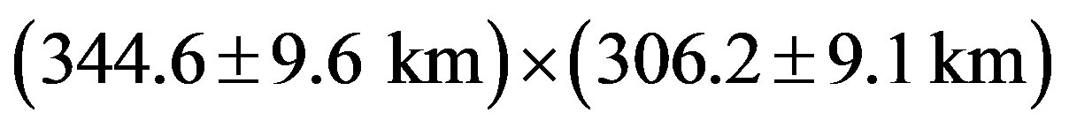whose posi

Table 1 . List of observed stellar occultations by (704) interamnia.

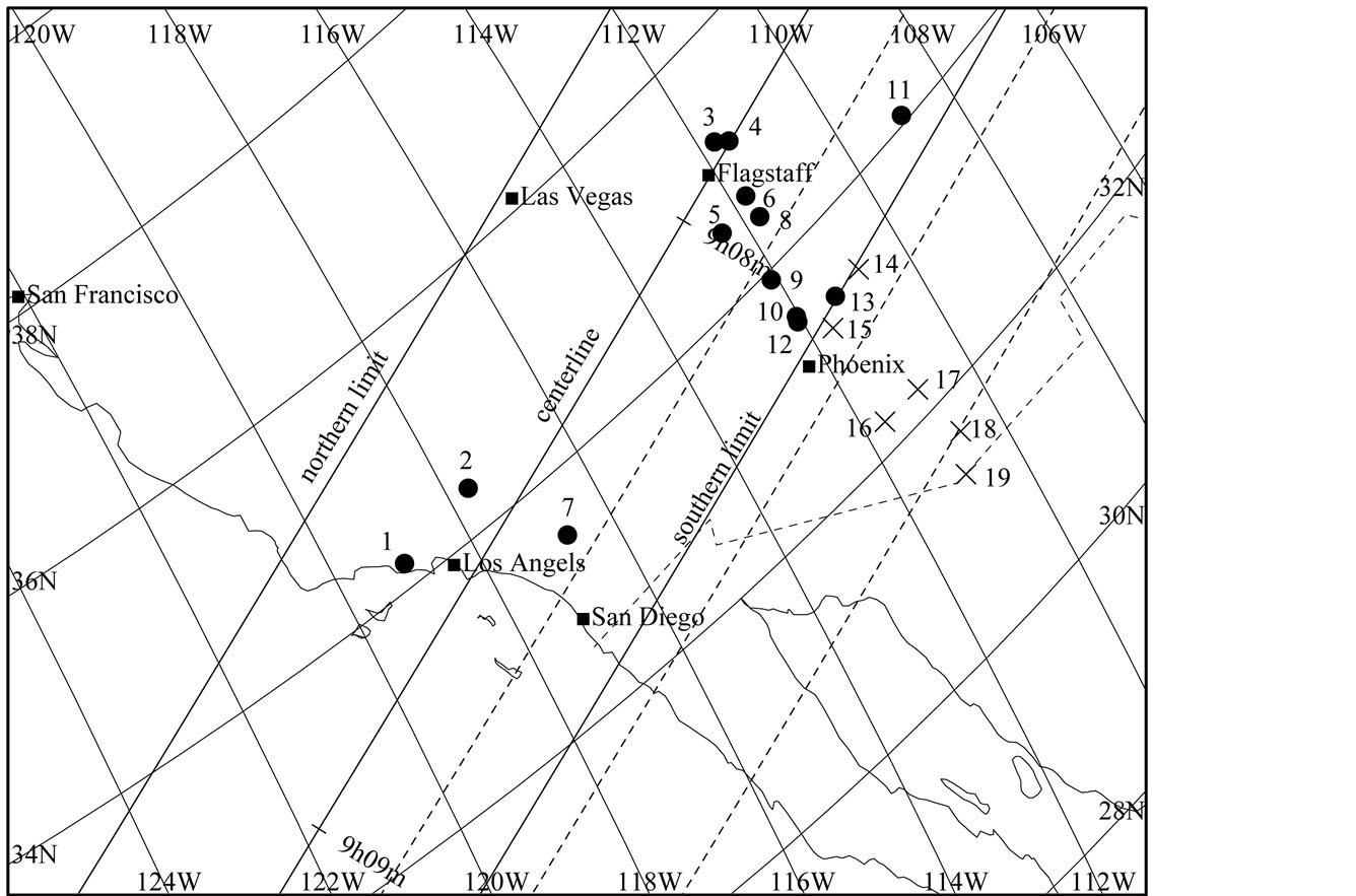
Figure 1. Local map of the occultation track and the locations of the observers in the USA for the 1996 December 17 event. The time is in UT. The observer numbers correspond to Table 2. indicates an occulted site (#1-13), and × indicates a no occultation site (#14-19). Solid lines indicate the actual occultation track, and dashed lines indicates the predicted occultation track.

tion angle 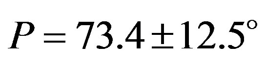is fitted by the weighted least squares method.

2.2. 2003 March 23 Event

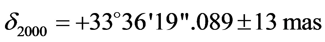
The occultation of HIP 036189 (= SAO 96908 = HD 58686 = BD + 12˚1548, , , m_v = 6.58) by (704) Interamnia on 2003 March 23 was predicted to be seen from Japan and Hawaii. Since Interamnia was nearly stationary as seen from Earth, the maximum duration of the extinction was over 70 seconds, very long for this kind of event.

Table 2. Observation data of the occultation of TYC234500183 by (704) Interamnia on 1996 December 17. Geodetic datum is WGS84.

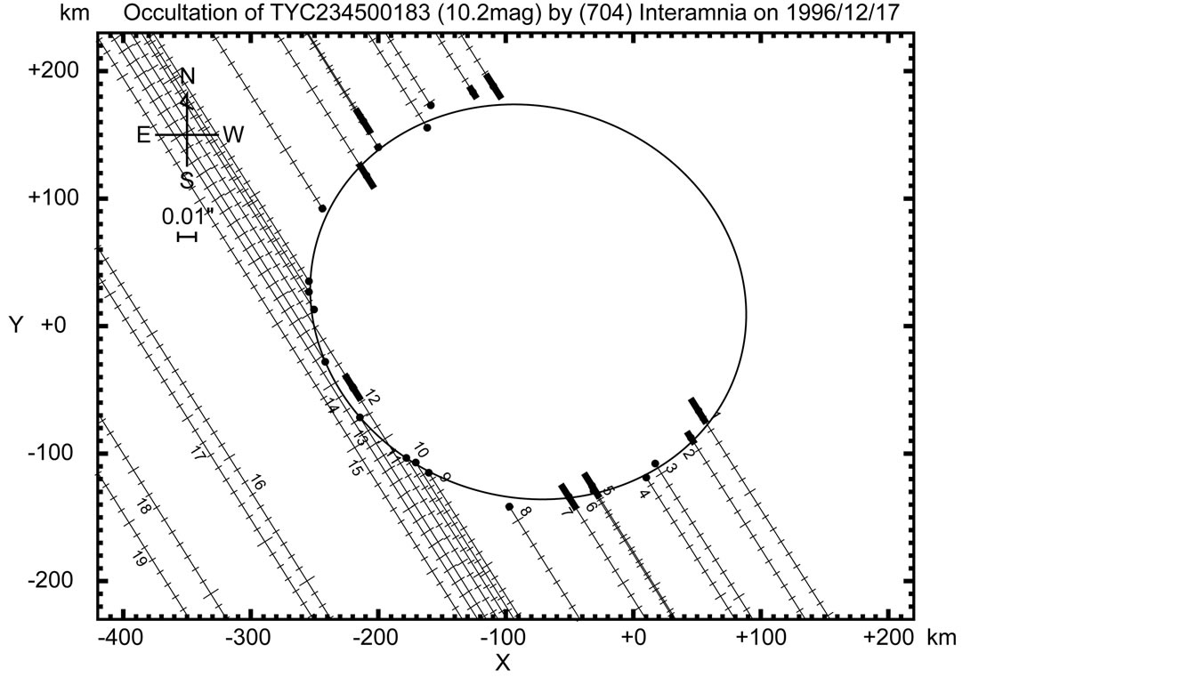
Figure 2. Occultation cross section of Interamnia obtained from the 1996 December 17 event. Size of the fitted ellipse is (344.6 ± 9.6 km) × (306.2 ± 9.1 km), P = 73.4 ± 12.5˚. The observer numbers correspond to Table 2. The star immerged from the southwest side, and emerged to the northeast side. The time interval of the tick mark of the star trace is one second. A solid dot is an absolute timed event, and an empty circle is a relative timed (time-shifted) event. The uncertainties of the timings are indicated by the thick lines associating the dots, for example #5.

Since Interamnia is a large asteroid, astrometric observations of this minor planet by meridian circles have been obtained since 1974. On the other hand, as for most faint asteroids, such high accuracy observations have been obtained just after 1997 when the USNO at Flagstaff, Arizona, USA, started an observation program of asteroids up to #2000 with CCD meridian circle instruments. This was very advantageous for Interamnia compared with other small asteroids.

Satō’s prediction was calculated using only these astrometric observations by the meridian circles and the HIPPARCOS satellite observations after 1985 adopted from the Minor Planet Center’s database. As a result, the nominal uncertainty of the ephemeris of Interamnia was reduced to just 9 mas compared with its angular diameter of 160 mas. The prediction is indicated as dashed lines in Figures 3, 4.

Fortunately, it was clear in both Japan and Hawaii on the day. Consequently, the event was observed from 24 sites in Japan and 15 sites in Hawaii. The observed occultation track and observation sites are shown in Figures 3, 4, and the observation results are listed in Table 3.

Although several observers (#7-15 in Figure 3) were located near the northern limit (predicted by Steve Preston) in Yamagata and Miyagi Prefectures (near Sendai) in Japan, the actual northern limit shifted to the south. So regrettably many observers saw no occultation just north of the actual northern limit. The shift of the actual occultation track compared to the predicted one is 18 mas south for Preston’s prediction, and 7 mas north for Satō’s prediction.

Isao Ohtsuki at Marumori, Miyagi, Japan, (#20) was located just on the northern limit. He recorded a onesecond gradual extinction by video observation. At the moment of immersion and emersion, the star light as a point source diffracts at the limb of the occulting body. The effect is called Fresnel diffraction. By this effect, the star does not disappear instantly but does so gradually. In the case of a point source, geometrical immersion or emersion corresponds to the time when the intensity decreses to 1/4 of the full intensity. Calculated Fresnel diffraction 1/4 time was 0.066 second in the case of perpendicular immersion or emersion. Also, the assumed angular diameter of the occulted star is 0.34 mas; hence, the partial duration in the case of perpendicular immersion or emersion was 0.133 second. In addition to these, a slant immersion effect along a very shallow

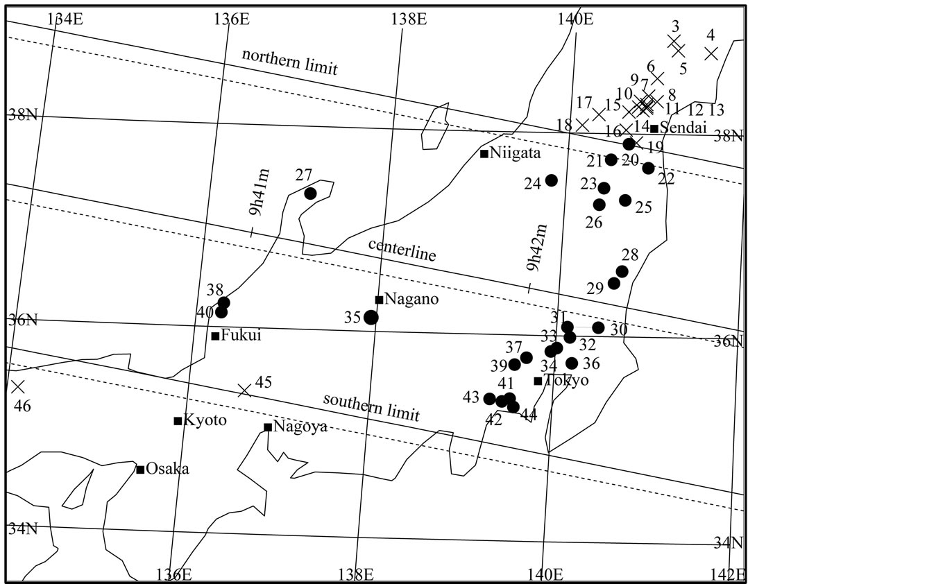
Figure 3. Local map of the occultation track and location of observers in Japan for the 2003 March 23 event. The time is in UT. Solid lines indicate the actual occultation track, and dashed lines indicate prediction occultaion track by Satō. The number of observers corresponds to Table 3. indicates an occulteded site (#20-44), and × indicates a no occultation site (#1-19, 45-46).

Figure 4. Local map of the predicted occultation track (Satō’s prediction) and location of observers in Hawaii on 2003 March 23. The time is in UT. Solid lines indicates the actual occultation track, and dashed lines indicates predicted occultaion track by Satō. The number of observers corresponds to Table 3. indicates an occulted site (#47-60).

Table 3. Observation data of the occultation of HIP036189 by (704) Interamnia on 2003 March 23 (Japanese observers). Geodetic datum is WGS84.

angle caused a long gradual extinction. The observed maximum duration of extinction was about 72 seconds. This is one of the longest records of asteroid occultations ever seen. Several observers located in the southern part of the occultation track reported double-stepped or gradual disappearance and reappearance by visual or video observations. These facts indicated the occulted star has a companion. The observed brightness of the companion was about 1.5 mag fainter than the primary. The existance of the companion had not been known.

The obtained cross section of Interamnia is shown in Figure 5. As the occulted star is double, two ellipses are displayed. The fitted ellipse is, position angle is and the separation of the companion is, position angle is.

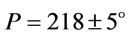3. Photometric Observations

3.1. Lightcurves before 1996

Lightcurves of Interamnia have been published five times between 1964 and 1993. De Angelis (1995) determined the pole solution in the ecliptic coordinates as 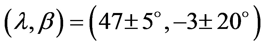or 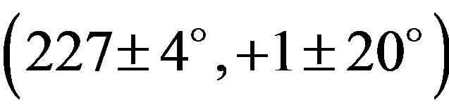using the data of Yang et al. (1965), Tempesti (1975), and Lustig & Hahn (1976) [9] [13] -[15] . Shevchenko et al.. (1992) reported photometric obsevations of Interamnia on 1990 August 1, but the coverage was just three hours [16] . Michalowski (1995) obtained a lightcurve of 0.11 mag amplitude from photometric observations in 1993, and he determined a pole solution as 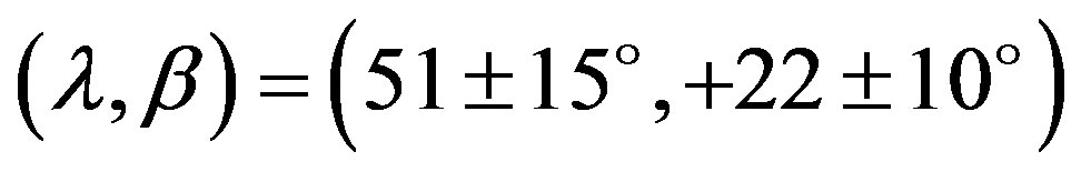[10] . We adopt four light-curves of Yang et al. (1965), Tempesti (1975), Michaowski et al. (1995), and our observations in the 3-D shape analysis. The mathematical formulation of the 3-D analysis is described in the Appendix of this paper.

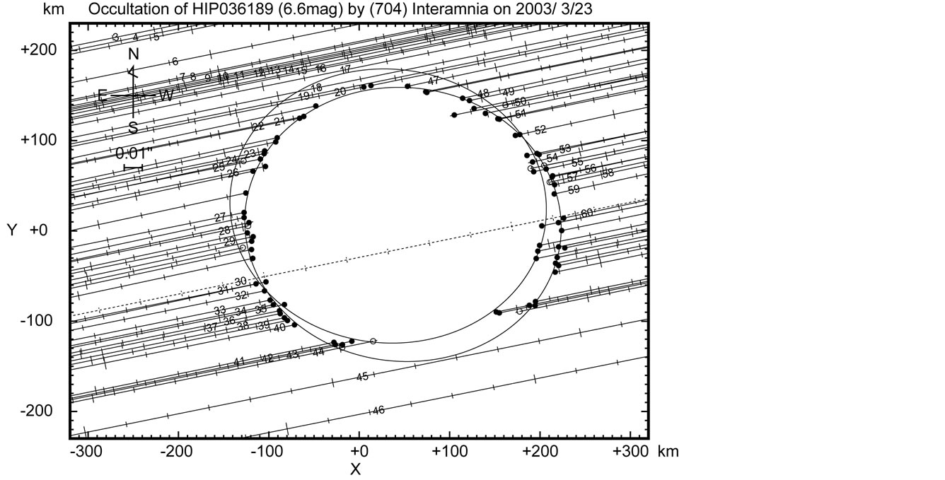
Figure 5. Occultation cross section of Interamnia obtained from the 2003 March 23 event. The star immerged into the east side, and emerged from the west side. The time interval of the tick mark of the star trace is 10 seconds. Since the occulted star HIP036189 is believed to be an unknown double, two same size ellipses are displayed for both the primary and the secondary star. The size of the fitted ellipse is (349.9 ± 1.1 km) × (303.5 ± 2.2 km), P = 85.8 ± 1.4˚. The separation of the binary is d = 12 ± 3 mas, P = 218 ± 5˚.

3.2. Lightcurve in 1996

A lightcurve obtained at Lowell Observatory on 1996 December 13 before the stellar occultation on December 17, is shown in Figure 6. The solid curve is a fifth order Fourier series fit assuming the rotation period 8.70 ± 0.06 hour [15] . The open squares around the rotation phase 0.9 show the phase of the occultation. The center square is the nominal phase and the outer two squares are at the phase for. The lightcurve shows peak-topeak amplitude of 0.04 mag, and the ocultation occured just before the second minimum. A tertiary maximum is shown earlier than the 0.15 rotation aspect. This light-curve structure supports the presence of topography on the object as seen in the limb fitted to the occultation chords.

3.3. Lightcurves in 2003

After the successful observation of the stellar occultation, follow-up photometry was performed with the 40 cm Newtonian telescope at Hamanowa Astronomical Observatory (MPC code = D91) and with the 60 cm Cassegrain telescope at Yanagida Astronomical Observatory (MPC code = 417). Generally speaking, the sky condition from Japan is not favourable for photometric observation because of the jet stream and changable weather. So the accuracy of the photometric observations of Interamnia was not so good.

Yanagida Astronomical Observatory observed Interamnia on 9 nights of 2003 March 20, 21, 22, 25, April 1, 3, 6, 10 and 15 (Figure 7). Hamanowa Astronomical Observatory observed Interamnia on 2003 March 18, 19, 21, 26, and April 3 (Figure 8). Each arrow in the figures indicates the time of the stellar occultation to show the occultation had occurred just after the lightcurve maximum. The solid sine curve in the figure shows the theoretical lightcurves derived from Equation (29); namely, it is proportional to the area of the cross section seen from the earth. The sine curve shows just the area of the cross section of the ellipsoid model, not including the effect of shadowing, albedo pattern, scattering property of the sunlight on the surface, and the deviation of the true shape of the asteroid from the ellipsoid model. So the difference between the sine curve and the observed lightcurve should be caused by these effects.

From these lightcurves, it is revealed that the sidereal rotation period was determined to be 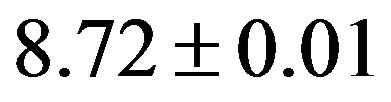hours (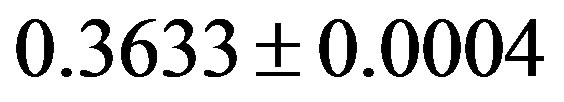days), the peak-to-peak amplitude was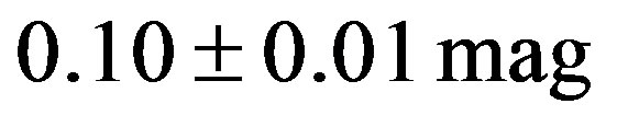, and the rotation phase at the

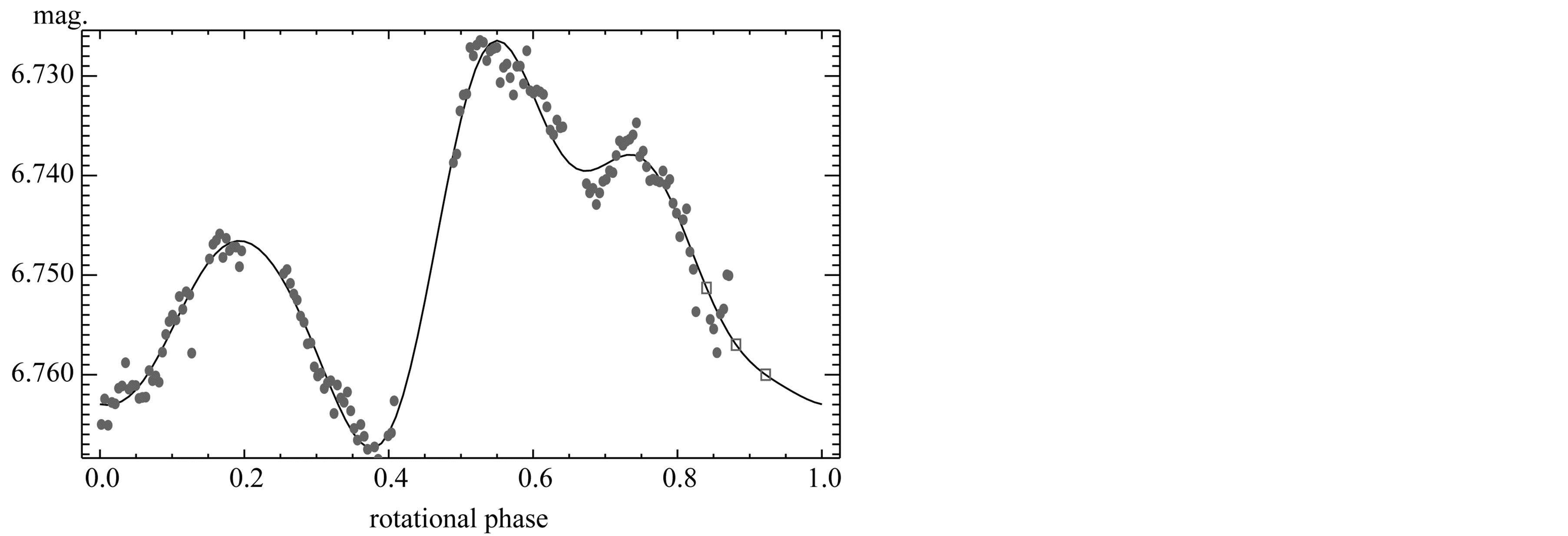
Figure 6. Lightcurve of Interamnia observed at Lowell Observatory on 1996 December 13. The rotational phase is relative to an arbitary epoch using the period derived from Lustig & Hahn (1976) data [14] . The solid curve is a fifth order Fourier series fit. The open squares show the rotational phase at the time of the occultation. The center is the nominal phase and the outer squares are at the phase for ±1σ from the best period.

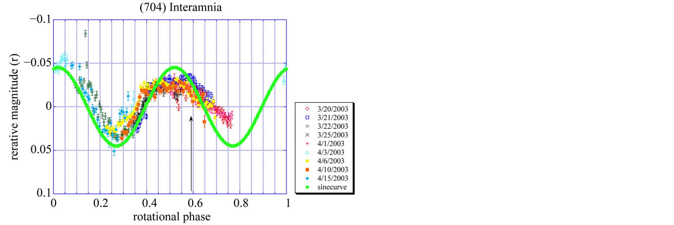
Figure 7. Lightcurve of Interamnia observed at Yanagida Astronomical Observatory from 2003 March 20 to April 15. Zero of the phase is 2003 March 18, 10h48m UT (2003 March 18.45000). The red vertical line indicates the time of the occultation, 2003 March 23, 9h42m UT (2003 March 23.40417). The solid sine curve is a theoretical lightcurve of the reproduced triaxial ellipsoid derived from Equation (29).

occultation was 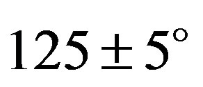from the minimum.

3.4. Lightcurve in 2011

As these lightcurves were obtained at the beginning stage of our photometric observation program, the accuracy of the observations was not satisfactory from the present point of view. Hence we again observed the asteroid at Hamanowa Astronomical Observatory. The photometric observation was performed on 2011 August 30, September 15, 16, 17, 18, 23, 24, and 25 (Figure 9). The accuracy of these observations is better than those in 2003 because the observation and reduction techniques are improved. The peak to peak amplitude was 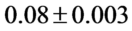mag. and the sidereal rotation period is 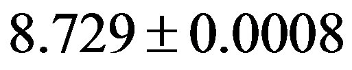hours. The total rotation period between 2003 and 2011 i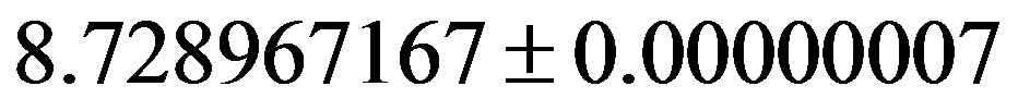s hours 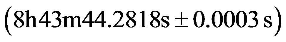in the sidereal period, and an epoch of a minimum is 2003 March 18.52917 (JD = 2452717.03002) UT in the true time.

Interamnia rotates about 8500 times between 2003 and 2011. Therefore if the number of rotations differs, derived rotation period differs 1.84 s per a half rotation. In order to fix the number of rotations, we checked the

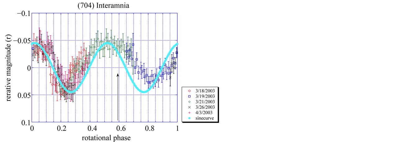
Figure 8. Lightcurve of Interamnia observed at Hamanowa Astronomical Observatory from 2003 March 18 to April 3. The epoch of the zero point of the rotation phase is 2003 March 18, 10h48m UT (JD = 2452716.95000). The rotation period is 8.72 ± 0.01 hours (0.3633 ± 0.0004 days) and full amplitude is 0.10 ± 0.01 mag. The arrow indicates the time of the occultation, 2003 March 23, 9h42m UT (2003 March 23.40417). The geocentric distance to Interamnia was 2.726692 AU, so the light time 0.01575 days should be corrected. Therefore the occultation occured at the rotational phase (23.40147 – 0.01575 – 18.45000)/0.36333 = 13 + 0.59211. The phase of the occultation is just after the maximum. The solid sine wave is a theoretical lightcurve of the model tri-axial ellipsoid derived from Equation (29). The difference between the theoretical lightcurve and the observed lightcurve shows the effects of the deviation from the ellipsoid model of the true shape of Interamnia, shadowing and albedo effect of the surface, and the backward scattering propery of the sunlight.

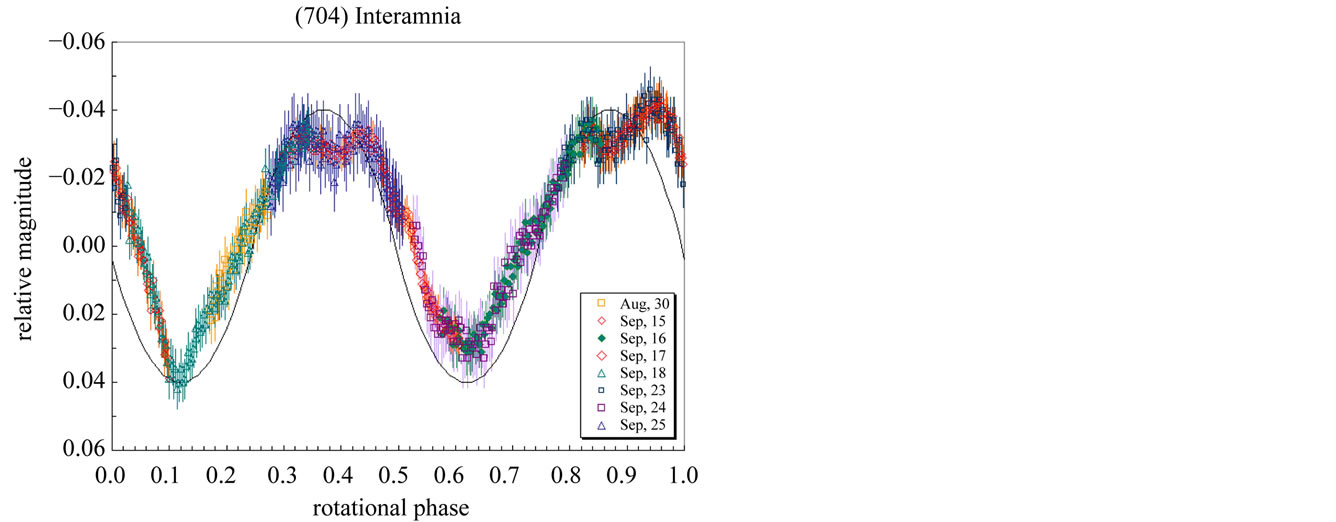
Figure 9. Lightcurve of Interamnia observed at Hamanowa Astronomical Observatory from 2011 August 30 to September 25. The origin of the rotation phase is 2011 August 30, 20h0m UT (JD = 2455803.33333). The solid sine wave is a theoretical lightcurve of the model tri-axial ellipsoid derived from Equation (29) whose rotation period is 8.729 ± 0.008 hours and the peak-to-peak amplitude is 0.08 ± 0.003.

fitness of the model to the four occultation cross sections of 1996, 2003, 2007, and 2009 events. As the result, only one rotation period among several cadidate rodation periods satisfies the all occultations cross sections. Above rotation period is determined in this way. The rotation period is accurate enough to reproduce the 3-D configurations of the asteroid at the past occultations uniquely. These reproduced situations will be discussed in the next section.

4. Result

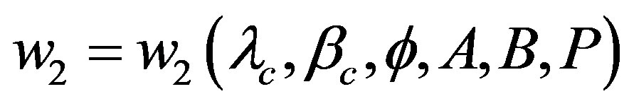
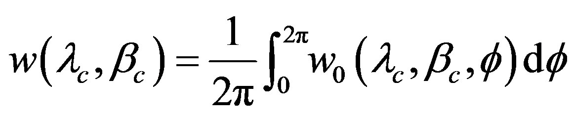
One occultation cross section gives just a weak constraint on the pole direction. Figure 10(a) shows a probability distribution of the spin vector derived from the occultation cross section on 2003 March 23 only. The density on the map indicates total likelihood of a triaxial ellipsoid model per square degree on the celestial sphere evaluated by the Equation (39) in the Appendix. If a spin vector is given at a grid, there are ellipsoid models of rotation phase between 0 to for each grid. Namely, the total volume of the phase space of parameters is. If there is no constraint on the model in a given spin vector, the density is unity. If there is no real solution of the model in a given spin vector, the density is zero. The density of each map is normalized between zero and the maximum value of each map. In general, when the constraint on the model by observation data is stronger, the maximum value on the map is lower. In the case of Figure 10(a), quarto symmetry distribution is shown [17] . This symmetry is originated from the symmetry of an ellipsoid model,

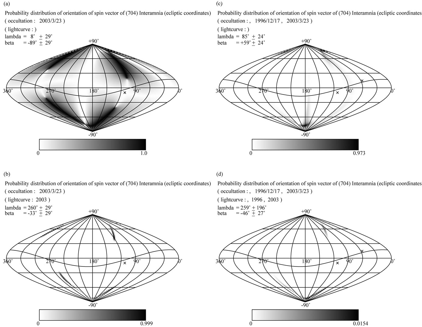
Figure 10. Probability distributions of the spin vector of Interamnia derived from selected occultation cross sections and lightcurves. The map is in ecliptic coordinates. The density of the map shows the likelihood per square degree derived from Equation (39). The gray scale is normalized between zero and the maximum value on the map of the density. The sine curve is the orbital plane of Interamnia, and two × indicate the location of the occulted stars of the 1996 and 2003 events, respectively. (a) is a probability distribution derived from the occultation cross section of the 2003 event only. (b) is a probability distribution derived from the occultation cross section and the lightcurve of the 2003 event. (c) is a probability distribution derived from the two occultation cross sections of the 1996 and 2003 events. (d) is a probability distribution derived from the two occultation cross sections and two lightcurves of the 1996 and 2003 events.

namely, a symmentry of rotation sense, prograde or retrograde, and a symmetry of hemispheres, the northern hemisphere and the southern hemisphere, or the eastern hemisphere or the western hemisphere.

If follow-up photometry of the asteroid after the stellar occultation is obtained, it could provide a greater constraint on it. Figure 10(b) shows a probability distribution of the spin vector derived from the occultation cross section and the lightcurve of the 2003 event. The probable region of the spin vector is strongly restricted compared to the case of an occultation cross section only (Figure 10(a)). If two occultation cross sections are obtained, the pole direction is restricted into two antipodal regions if accurate enough. Figure 10(c) shows a probability distribution of the spin vector derived from the two occultation cross sections of the 1996 and the 2003 events. The probable region of the spin vector is fairly different from Figure 10(b). If two occultation cross sections and one or more lightcurve(s) are obtained, a unique solution of the pole is determined if accurate enough. Figure 10(d) shows a probability distribution of the spin vector derived from the two occultation cross sections of the 1996 and the 2003 events, and the lightcurves in 1996 and 2003. If more observations are obtained, the pole and 3-D shape of the asteroid would be constrained more strongly. Figure 11 shows the final result of the probability distribution of the spin vector derived from two occultation cross sections of 1996 and 2003 events, and six lightcurves.

In Figures 10 and 11, the densities of the maps show the likelihood per square degree derived from Equation (39). The gray scale is normalized between zero and the maximum value on the map of the density. The maximum value of the density is unity; namely, the entire range of the rotation phase angle (0 to) has a real solution. The map is in ecliptic coordinates, and the sine curve indicates the orbital plane of Interamnia. Figure 11 shows the most probable spin vector is at, , around Triangulum Australe, namely retrograde rotation.

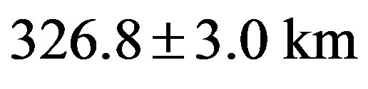
Figure 12 shows the probability distribution of the lengths of the three principal axes. The derived values are, and the mean diameter is . The ratios of the three principal axes are 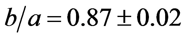and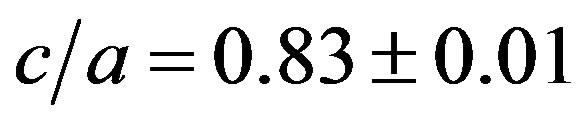. Figures 13 and 14 show the reproduced occultation cross sections of the 1996 and 2003 events, respectively.

In order to verify the 3-D model of Interamnia, some occultation cross sections of the past events are repro-

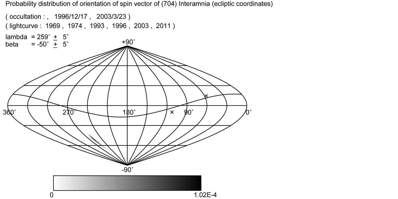
Figure 11. Probability distributions of the spin vector of Interamnia derived from two occultation cross sections and six lightcurves. The map is in ecliptic coordinates. The density of the map shows the likelihood per square degree derived from Equation (39). The gray scale is normalized between zero and the maximum value on the map of the density. The sine curve is the orbital plane of Interamnia, and two × indicate the location of the occulted stars of 1996 and 2003 events, respectively. The most probable spin vector is λ = 259 ± 5˚, β = −50 ± 5˚. This is around Triangulum Australe.

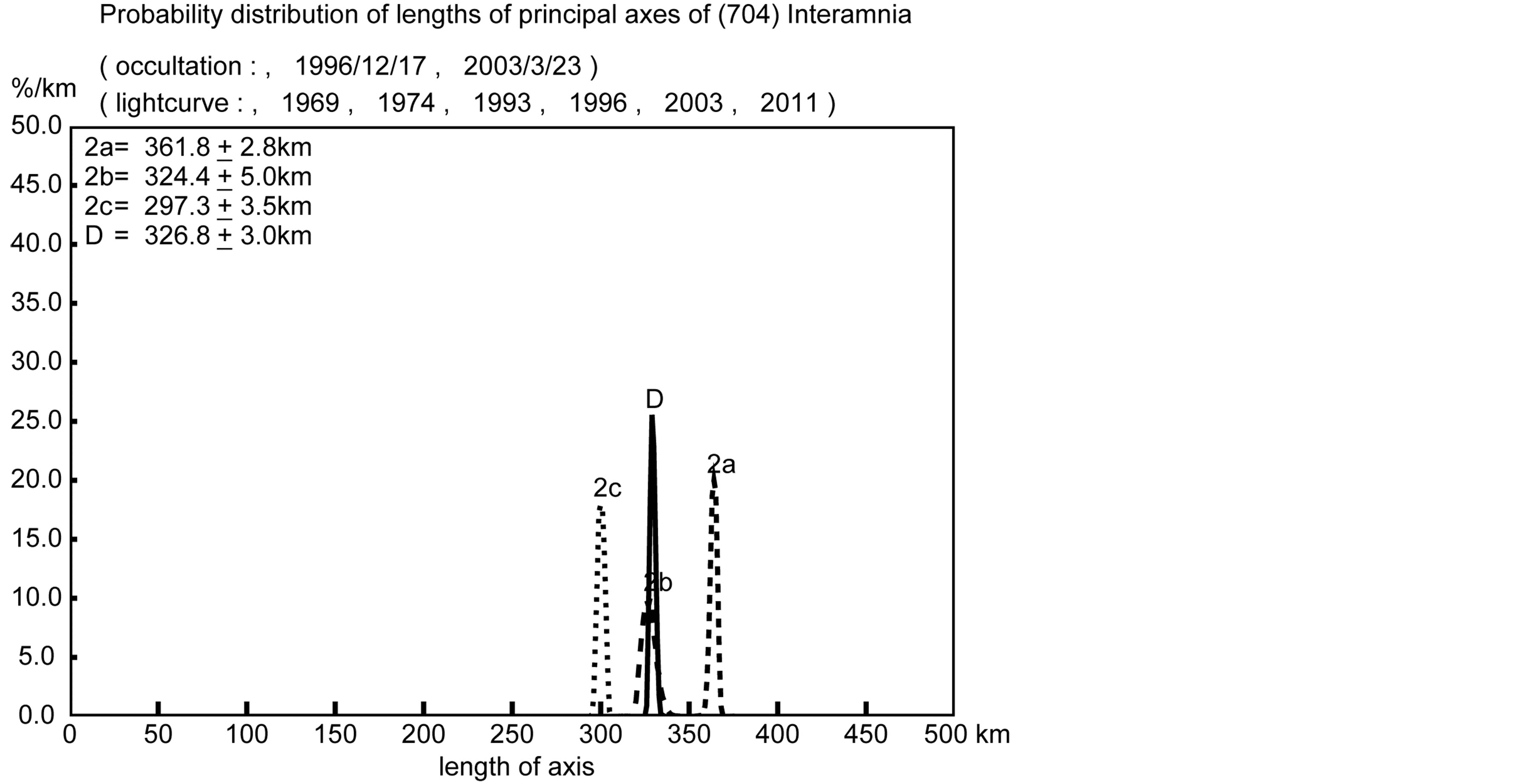
Figure 12. Probability distributions of the three principal axes a, b, c and the mean diameter D of Interamnia derived from the two occultation cross sections and all lightcurves. Each distribution shows a sharp peak suggesting a good solution. The most likely solution is 2a = 361.8 ± 2.8 km, 2b = 324.4 ± 5.0 km, 2c = 297.3 ± 3.5 km, and D = 326.8 ± 3.0 km.

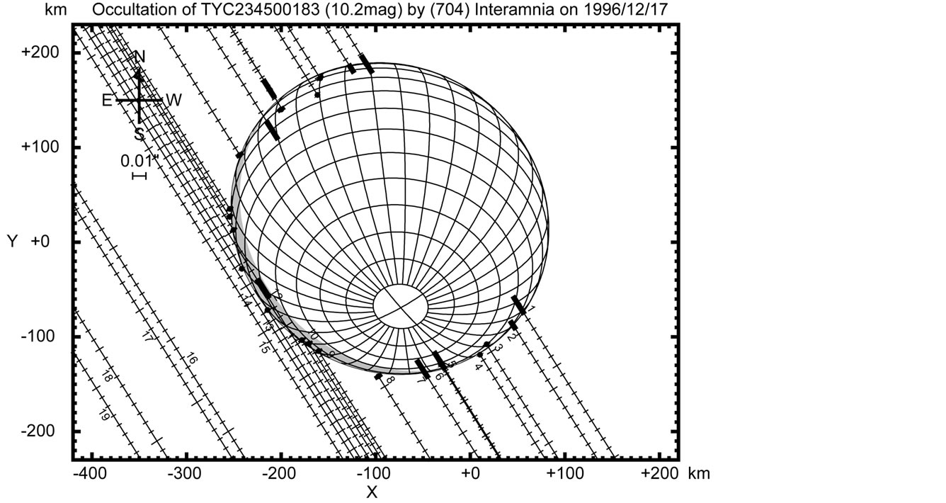
Figure 13. Reproduced occultation cross section of Interamnia at the 1996 December 17 event. The grid is every 10 degrees in longitude and latitude, respectively. The shaded area indicates the night side. The observer numbers correspond to Table 2. The star merged into the southwest side, and emerged from the northeast side. The time step of the star trace is one second. The uncertainties of the timings are indicated by the thick lines associating the dots, for example #4.

duced. The rotation phases at the stellar occultations are assumed from our rotation period. Figures 15-16 show the reproduced cross sections at the stellar occultations on 2007 September 9, and 2009 January 11, respectively (See Table 1).

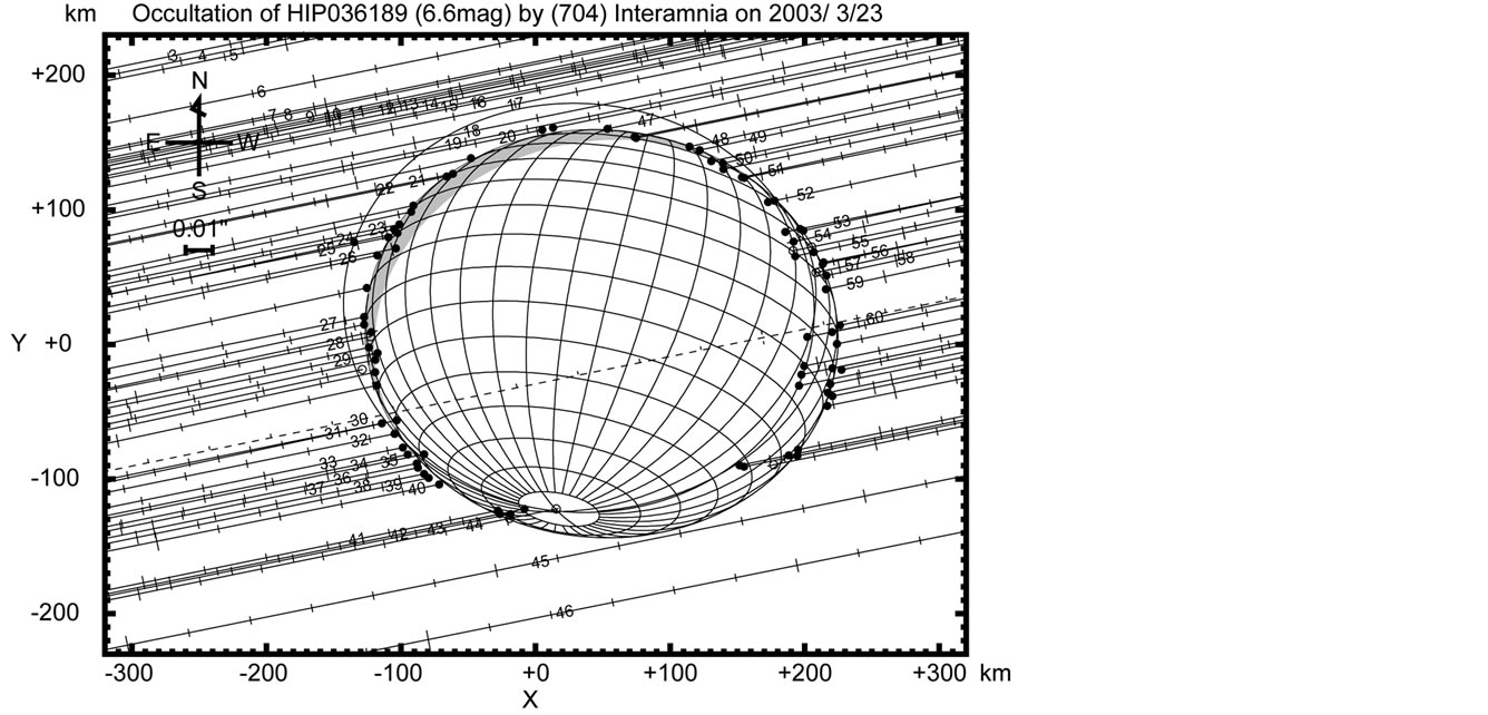
Figure 14. Reproduced occultation cross section of Interamnia at the 2003 March 23 event. The grid is every 10 degrees in longitude and latitude, respectively. The shaded area indicates the night side. The star immerged from the east side, and emerged to the west side. The time interval of the star trace is 10 seconds. Since the occulted star HIP036189 is an unknown double, two same size ellipses are displayed for both the primary and secondary star. The separation of the binary is d = 12 ± 3 mas, P = 218 ± 5˚.

Although enough occultation chords to fit an elliptical cross section were not obtained at these events, the reproduced configurations from our model coincide well with the observations. Therefore we have high confident in the model.

The mass of Interamnia has been determined as 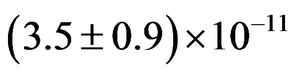solar mass [18] . From the obtained mean diameter, the mean density is determined to be (3.8 ± 1.0) g∙cm⁻³. The density is high compared with other main belt asteroids and near Earth asteroids, (4) Vesta is (3.4 - 3.5) g∙cm⁻³, (2) Pallas is (2.6 - 3.1) g∙cm⁻³, are comparable, but most of other smaller asteroids are less dense [19] .

5. Discussion

Michalowski (1993) determined the first solution of the pole of Interamnia as, or with probable retrograde rotation [20] . De Angelis (1995) determined the new pole as

, or [9] . Michaowski (1995) improved the pole using a new lightcurve in 1993 as with prograde rotation [10] . These previous results are based on the lightcurves only. Although our solution is quite different from these previous results, our result contains information about the absolute orientation of Interamnia through the two occultation cross sections. The reproduced 3-D shape of Interamnia fits the several occultation cross sections well.

The assumed diameter was derived from 10 sighting observations made by IRAS in the period of from 13 July to 28 August, 1983 [6] . In order to discuss the difference of the diameters, we reproduce these situations from our model (Figure 17). Table 4 shows the reproduced cross sections at the 10 IRAS observations. The total mean diameter of the 10 cross sections is 328.7 km. The value is not so biased compared with the mean diameter 326.8 ± 2.8 km of our model, but the assumed diamter 317 ± 5 km is significantly (3.0%) smaller than this value. Reanalysis of 10 IRAS observations with NEATM gives 334 ± 14 km [21] . This value is not significantly different from our model. Therefore NEATM is supported by our result.

6. Conclusion

From the combination of the two occultation cross sections and six lightcurves, a new tri-axial ellipsoid model

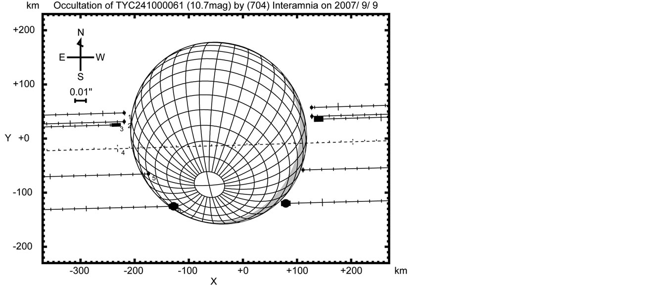
Figure 15. Reproduced occultation cross section of Interamnia at the 2007 September 9 event observed from six sites in USA (#4 site is untimed). The coverage of the occultation chords was not enough to fit an ellipse cross section, but the reproduced profile is not discrepant with the observed profile.

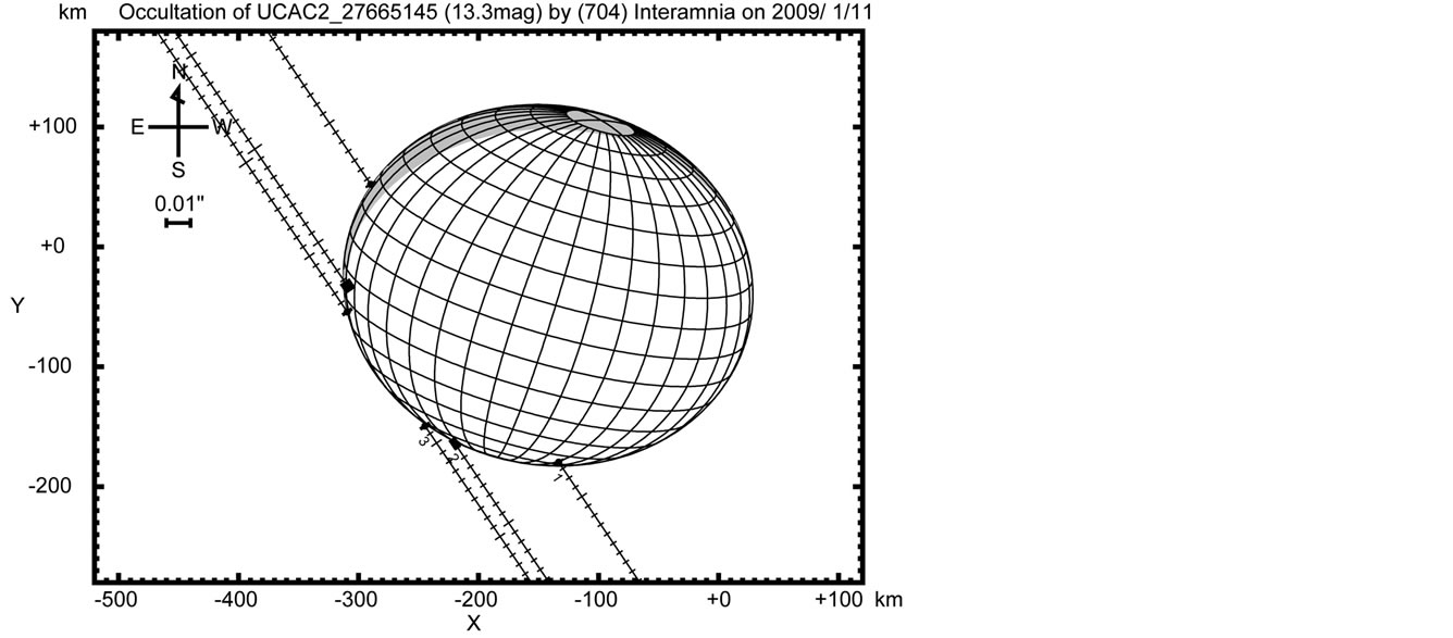
Figure 16. Reproduced occultation cross section of Interamnia at the 2009 January 11 event observed from three sites in France. The coverage of the occultation chords was not enough to fit an elliptical cross section, but the reproduced cross section is not discordant with the observations.

Table 4. Rotation phases of (704) Interamnia at the times of occultation observations and photometric obervations. τ is the light time between Interamnia and the earth in seconds which is to be corrected for the true and apparent rotation phase angles. The rotation phase ϕ and ϕ₀ are the apparent and the true phase angle since 2003 March 23.4500 (UT) supposing the rotation period 8.728967167 ± 0.00000007 hours, respectively. θ is the phase angle from a lightcurve minimum. n_rot is the times of rotation counted from the 2003 March 23, 09h42m (UT).

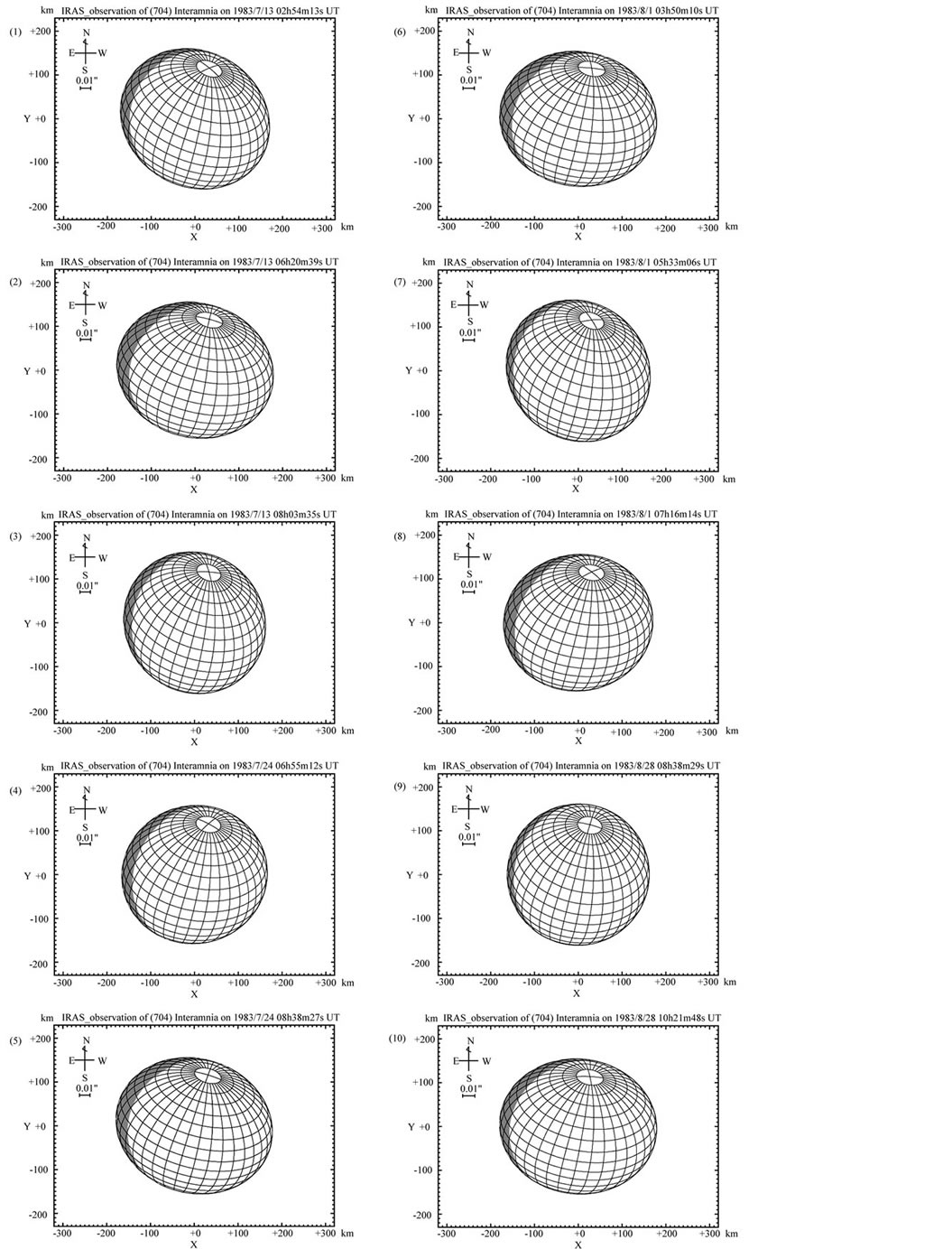
Figure 17. Reproduced cross sections of Interamnia at the times of 10 IRAS observations on 1983 July 13, 24, August 1, and 28. The detail of the situations is shown in Table 5. The average of the mean diameters of the 10 cross sections is 327.2 km, compared with the mean diameter of 328.7 ± 2.3 km of our model. The assumed diameter of 317 ± 5 km [6] is significantly smaller than this value, but the new value 334 ± 14 km by NEATM [20] is coincident.

Table 5. List of the reproduced cross section of (704) Interamnia at the times of IRAS observations. The rotation phase is the apparent phase angle since 2003 March 23.4500 (UT) supposing the rotation period 8.728967167 hours. The Δ mag. is the relative brightness to the maximum cross section derived from our 3-D model. The total mean diameter at the observations is 328.7 km.

of Interamnia has been obtained. The pole is around Triangulum Australe indicating a retrograde rotation. This pole is very different from previous results. The lengths of the three principal axes have been also obtained to an excellent level of accuracy. From the mass of Interamnia, its density has been derived.

This is an excellent result of a 3-D shape model obtained from asteroid occultations and lightcurves. Thanks to efforts by many people all over the world, we have achieved a unique result, which has been a goal since G. E. Taylor first recognized the potential of asteroid occultations in 1952.

References

Taylor, G.E. (1952) Occultations of Stars by Asteroids. Handbook of the British Astronomical Association for 1953, The University of Chicago, Chicago.
Taylor, G.E. (1962) Diameters of Minor Planets. Notes from Observatories, 926, 17.
Sinvhal, S.D., Sanwal, N.B. and Pande, M.C. (1962) Observation of the Occultation of BD−5˚5886 by Pallas. Notes from Observatories, 926, 16-17.
Millis, R.L., Wasserman, L.H., Bowell, E., Franz, O.G., Klemola, A. and Dunham, D.W. (1984) The Diameter of 375 Ursula from Its Occultation of AG +39˚303. Astronomical Journal, 89, 592-596. http://dx.doi.org/10.1086/113553
Satō, I., Šarounova, L. and Fukushima, H. (2000) Size and Shape of Trojan Asteroid Diomedes from Its Occultation and Photometry. Icarus, 145, 25-32. http://dx.doi.org/10.1006/icar.1999.6316
Tedesco, E.F., Noah, P.V., Noah, M. and Price, S.D. (2002) The Supplemental IRAS Minor Planet Survey. Astronomical Journal, 123, 1056-1085. http://dx.doi.org/10.1086/338320
Tholen, D.J. (1984) Asteroid Taxonomy from Cluster Analysis of Photometry. Ph.D. Thesis, University of Arizona, Tucson.
Hiroi, T., Peters, C.M. and Zolensky, M.E. (1983) Comprison of Reflectance Spectra of C Asteroids and Unique C Chondrites Y86720, Y82162, and B7904. Proceedings of 24th Lunar and Planetary Science Conference, Part 2 G-M, 659-660.
De Angelis, G. (1995) Asteroid Spin, Pole and Shape Determinations. Planetary and Space Science, 43, 649-682. http://dx.doi.org/10.1016/0032-0633(94)00151-G
Michalowski, T., Velichko, F.P., Di Martino, M., Krugly, Y.N., Kalashnikov, V.G., Shevchenko, V.G., Birch, P.V., Sears, W.D., Denchev, P. and Kwiatkowski, T. (1995) Models of Four Asteroids: 17 Thetis, 52 Europa, 532 Herculina, 704 Interamnia. Icarus, 118, 292-301.
Buie, M.W., Wasserman, L.H., Millis, R.L., White, N.M., Nye, R., Dunham, E.W., Bosh, A.S., Stone, R., Hubbard, W.B., Hill, R., Dunham, D.W., Fried, R., Kilinglesmith, D., Sanford, J., Schwaar, P., Maley, P., Owen, W., Benner, L., Rivken, A.S., Spitale, J., Marcialis, R.L. and Lebofsky, L.A. (1997) Occultation of GSC 23450183 by (704) Interamnia on 1996 December 17. Bulletin of the American Astronomical Society Abstract, No. 29, 973.
Wasserman, L.H. (1997) Occultations and Asteroids: The Rest of the Story. Lowell Observers, 35, 2-4.
Yang, X.Y., Zhang, Y.Y. and Li, X.Q. (1965) Photometric Observations of Variable Asteroids III. Acta Astronomica Sinica, 13, 66-74.
Tempesti, P. (1975) Photoelectric Observation of the Minor Planet 704 Interamnia during Its 1969 Oppositions. Memorie della Societa Astronomica Italiana, 46, 397-405.
Lustig, G. and Hahn, G. (1976) Photoelektrische Lichtkuven der Planetoiden 2 Pallas und 704 Interamnia. Acta Physica Austriaca, 44, 199-205.
Shevchenko, V.G., Chiornija, V.G., Kruglya, Y.N., Lupishkoa, D.F., Mohameda, R.A. and Velichkoa, F.P. (1992) Photometry of Seventeen Asteroids. Icarus, 100, 295-306. http://dx.doi.org/10.1016/0019-1035(92)90102-D
Satō, I., Sôma, M. and Hirose, T. (1993) The Occultation of Gamma Geminorum by the Asteroid 381 Myrrha. Astronomical Journal, 105, 1553-1561. http://dx.doi.org/10.1086/116535
Michalak, G. (2001) Determination of Asteroid Masses: II. (6) Hebe, (10) Hygiea, (15) Eunomia, (52) Europa, (88) Thisbe, (444) Gyptis, (511) Davida, and (704) Interamnia. Astronomy & Astrophysics, 374, 703-711. http://dx.doi.org/10.1051/0004-6361:20010731
Hilton, J.L. (2002) Asteroid Masses and Densities, Asteroids III. University of Arizona Press, Tucson, 103-112.
Michalowski, V. (1993) Poles, Shapes, Senses of Rotation, and Siderial Period of Asteroids. Icarus, 106, 563-572.
Harris, A.W. (1998) A Thermal Model for Near-Earth Asteroids. Icarus, 131, 291-301. http://dx.doi.org/10.1006/icar.1997.5865
Stamm, J. (1984) Occultation Newsletter, 3, 185.
Stamm, J. (1991) Occultation Newsletter, 5, 93.
Satō, I. (1996) Asteroid Occultation Observations from Japan. Doctoral Thesis at the Graduated University for Advanced Studies, 163.
Dunham, D.W., et al. (2013) http://sbn.psi.edu/pds/asteroid/EAR_A_3_RDR_OCCULTATIONS_V11_0/

7. Appendix: Mathematical Formulation of 3-D Shape Analysis

An occulation cross section gives a constraint to the direction of the pole and 3-D shape of the occulting asteroid. The first work to reconstruct a 3-D shape was made by an author for the case of the occultation of Geminorum by (381) Myrrha [16] . Follow-up photometry accompanying an occultation gives further constraint to the pole direction and 3-D shape [5] .

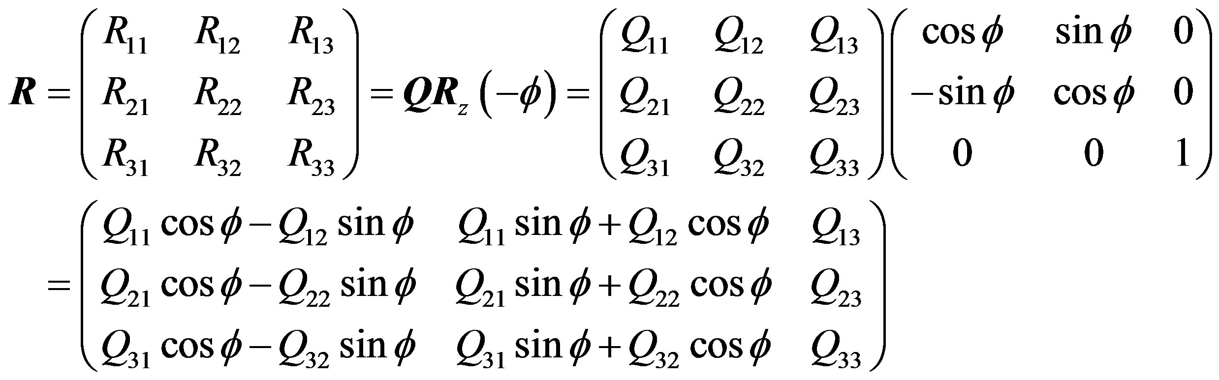
Supposing a tri-axial ellipsoid, an occultation cross section is an ellipse defined by the projection of the ellipsoid to a plane being perpendicular to the line connecting the center of the ellipsoid to the star and passing through the center of the ellipsoid. If two occultation cross sections and one lightcurve of the asteroid are obtained with enough accuracy, a unique 3-D shape model of the asteroid can be determined. However, no such work has been done. As for Interamnia, two occultation cross sections have been obtained. Especially, one of the two, the 2003 event, is very excellent. Therefore a 3-D shape analysis can be performed with a lightcurve to determine a unique model.

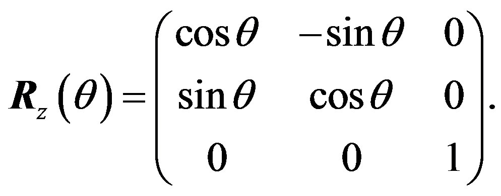
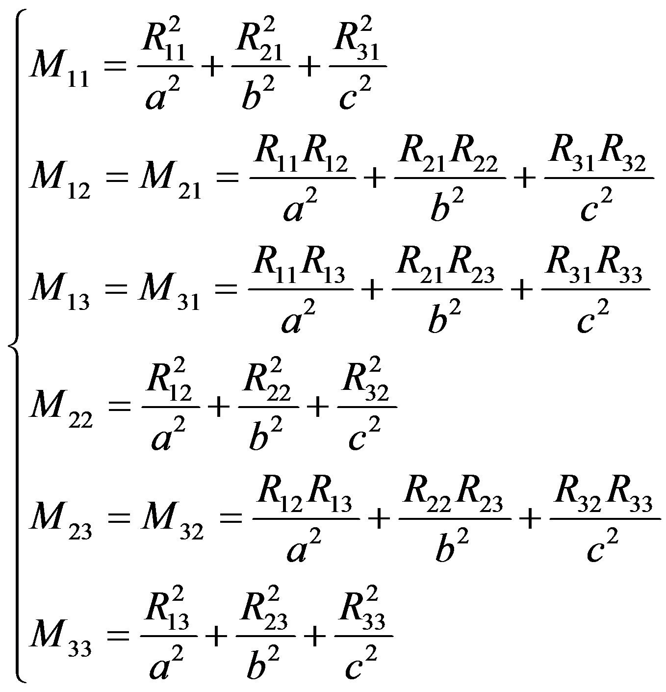
A configuration of a tri-axial ellipsoid is described by seven parameters: half lengths of the three principal axes, direction of the north pole in the ecliptic coordinates, rotation phase angle of the a-axis around the c-axis measured from the ascending node with the ecliptic plane, and rotation period. If are supposed, three principal axes are determined uniquely by an occultation cross section [16] .

Since the three angle parameters are finite, namely, , , the whole volume of the phase space in the three dimensions is finite. If are given, we can test if the ellipsoid model can yield another occultation cross section by changing from 0 to. If a satisfactory exists, it becomes a possible 3-D model for the given. However, such a solution does not exist in general.

Two occultation cross sections provide six constraints for six parameters except for the rotation period p. Therefore one set of antipodal pole directions can be determined by two occultation cross sections. In order to determine whether the rotation is prograde or retrograde, the rotational phase at the time of the occultation is required. If three or more occultation cross sections and/ or two or more lightcurves are obtained, uncertainty of the solution can be reduced by statistical methodology such as the least square or the most likelihood.

A standard form of a tri-axial ellipsoid is

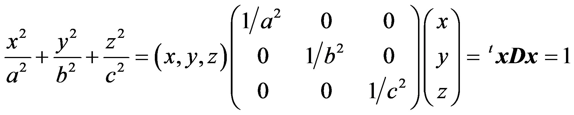(1)

where

(2)

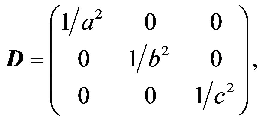(3)

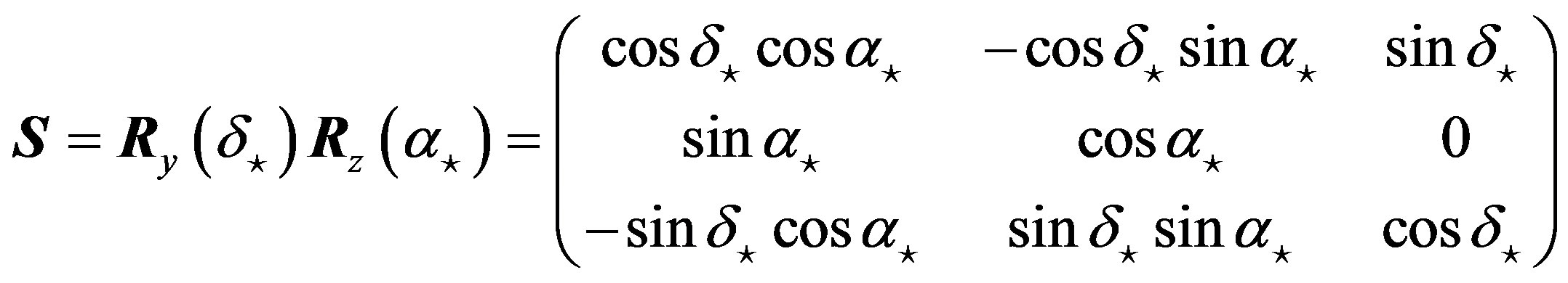
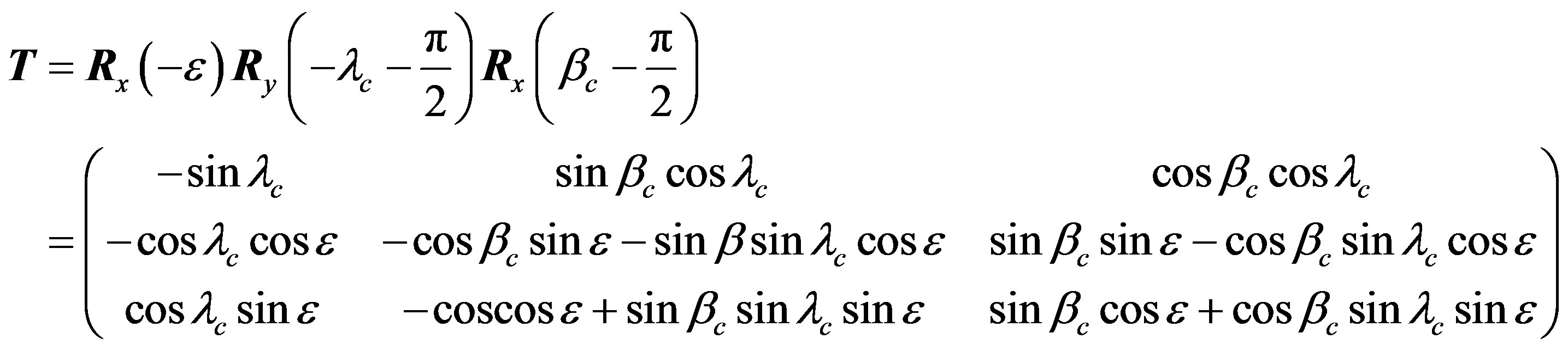
is defined by the ecliptic coordinates by

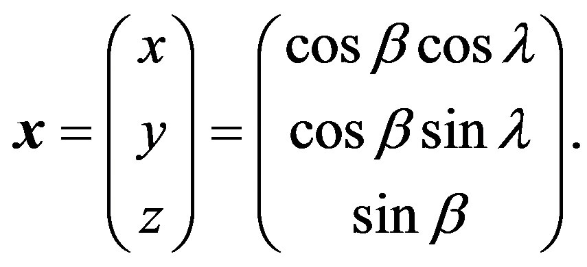(4)

Namely, the x-axis is toward the vernal equinox, the y-axis is toward the summer solstice point, and the z-axis is toward the ecliptic north pole.

As is illustrated in Figure 18, assuming the rotation axis being equivalent to the c-axis, in the case that the direction of the rotation axis is, , and the rotation phase angle is,

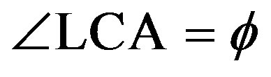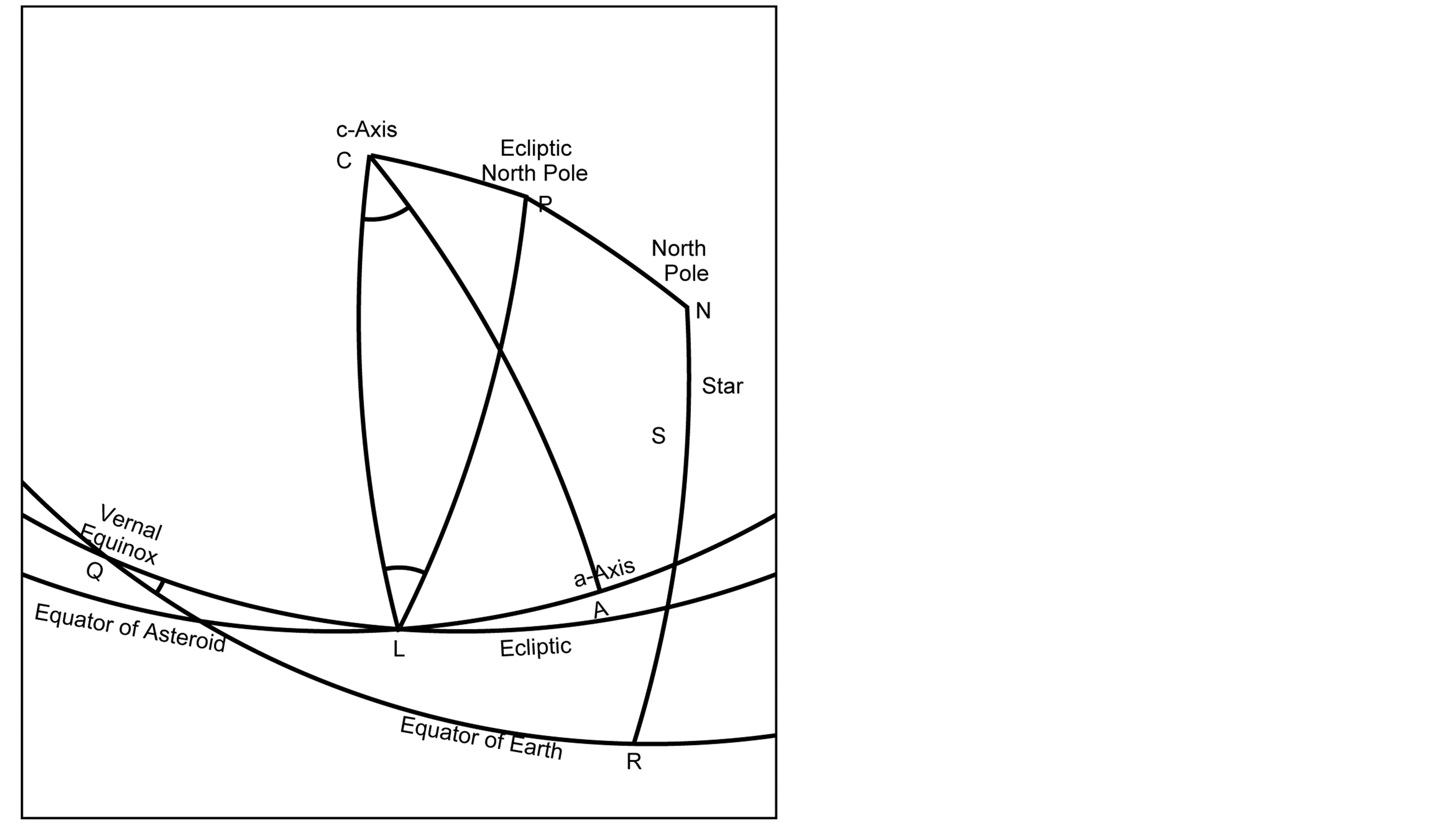
Figure 18. Explanation of the definitions of the parameters used in the Appendix. The north pole is N, the ecliptic north pole is P, the Vernal equinox is Q, the c-axis of the model ellipsoid is C being equivalent to the rotation axis, the a-axis of the ellipsoid is A, the occulted star is S, the ascending node of the equator of the asteroid is L, the ecliptic obliquity is, the ecliptic longtude and the latitude of the c-axis are and, respectively, the rotation angle of the a-axis is, the right ascension and the declination of the occulted star are and respectively.

at first, the ellipsoid should be rotated around the z-axis. Second, rotate around the x-axis. Third, rotate around the new z-axis.

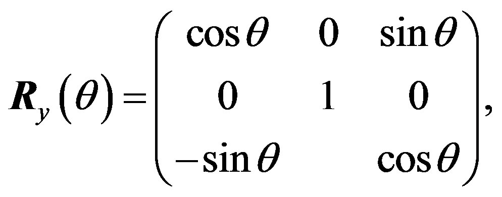
Since the direction of the asteroid (and the occulted star) seen from the observer is expressed in the equatorial coordinates in the usual case, rotate around the new x-axis in order to convert from the ecliptic coordinates to the equatorial coordinates, where 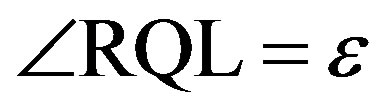is the ecliptic obliquity. Then rotate QR = around the z-axis, and rotate around the y-axis. Therefore the total rotation matrix is

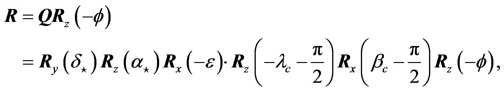(5)

where, , are rotation matrices around each axis,

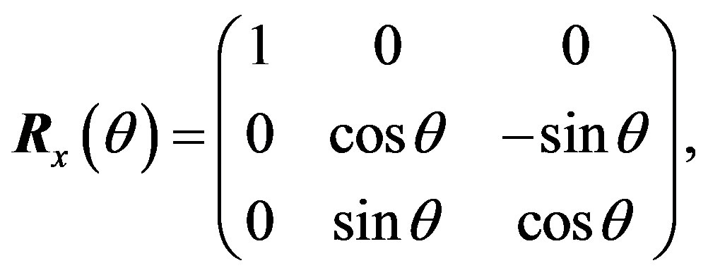(6)

(7)

(8)

The components of 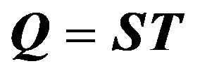are given as follows,

(9)

(10)

Components of are

(11)

where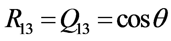, is the aspect angle, the angle between observer’s line of sight and the rotation axis [21] . is a constant matrix with respect to the rotation of the asteroid.

According to above result, a general form of a tri-axial ellipsoid is written as follows,

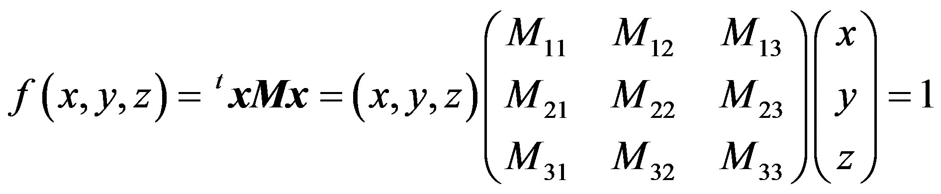(12)

where the matrix is given as follows,

(13)

(14)

Also, as in Equation (1), a standard form of an ellipse is given by

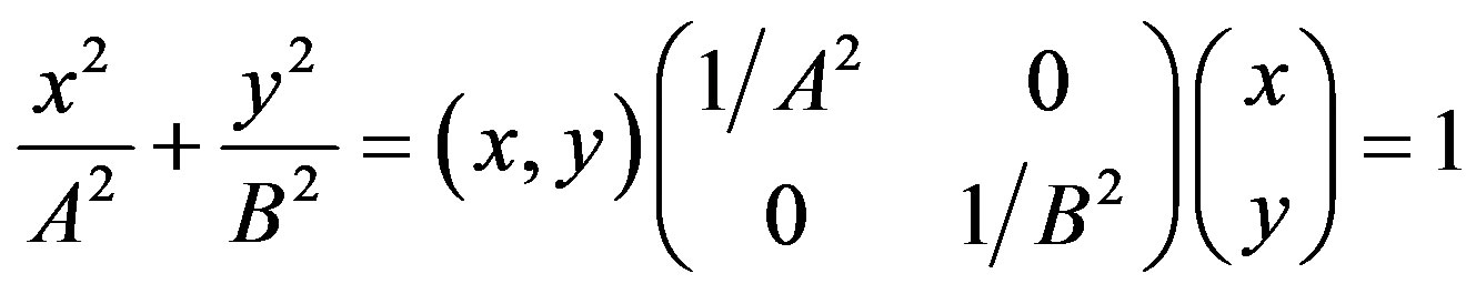(15)

where A and B are the observed semi-major and the semi-minor axes of the ellipse, respectively.

An ellipse as an occultation cross section is a projection of the tri-axial ellipsoid on the plane perpendicular to the line connecting the center of the ellipsoid to the star and passing through the center of the ellipsoid. On the outline of the apparent cross section of the tri-axial ellipsoid, its tangential plane is parallel to the line of sight. Therefore, in the case of projection from the x-axis direction, the apparent cross section of the tri-axial ellipsoid is obtained by solving the Equation (12) and its partial equation following, simultaneously,

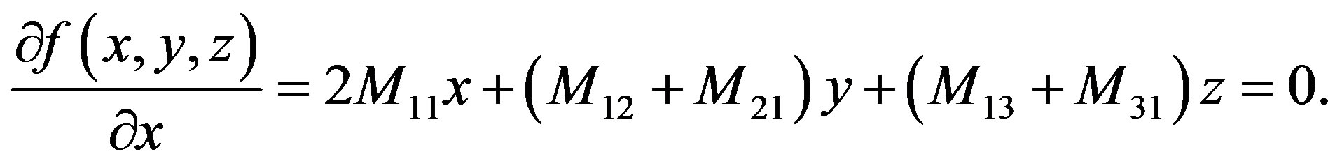(16)

From the above equation, we have

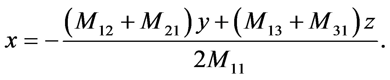(17)

Substituting this into Equation (12), we have

(18)

where

(19)

Substituting Equation (14) into above equations, we have

(20)

where is

(21)

In the above calculation, since is an orthogonal matrix, its adjugate matrix is equal to its transpose matrix and its inverse matrix. Namely,

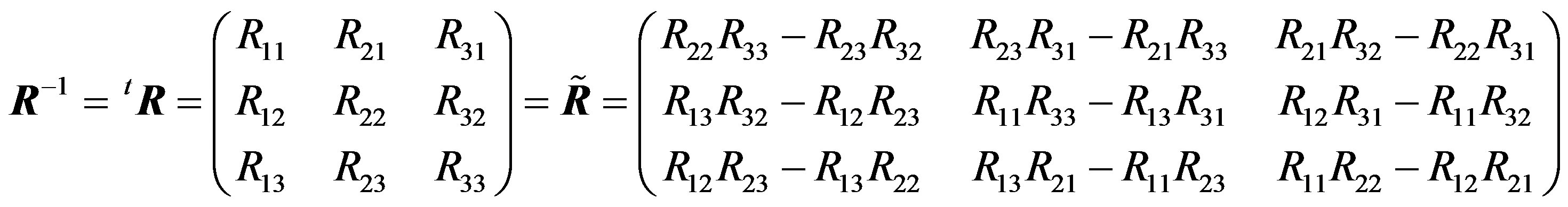(22)

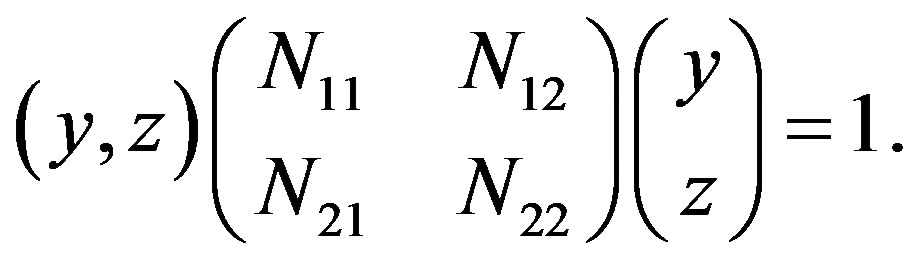
Since the observed lengths of the major and the minor axes of the apparent cross section are 2A and 2B, they are given as the eigenvalues λ₁, λ₂ of the matrix N. Namely,

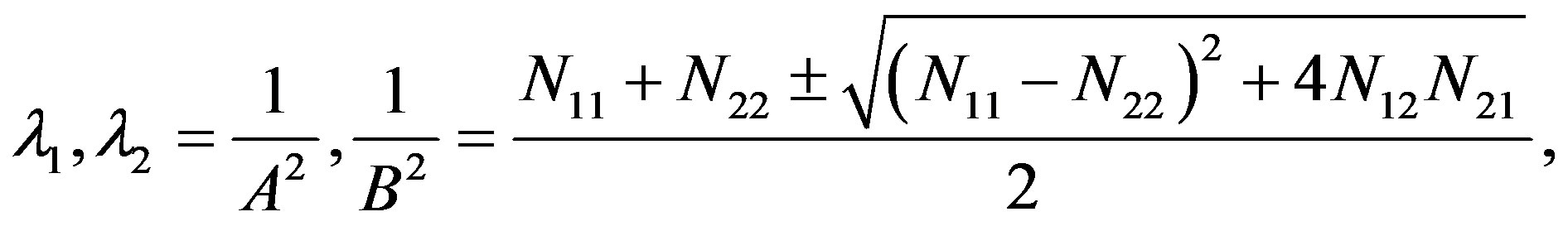(23)

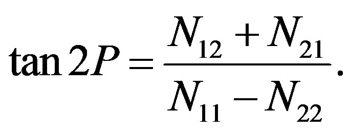(24)

where P (not the rotation period p) is a position angle (measured east-ward from the north pole) of the A-axis. As is shown above, we obtained a cross section of the asteroid. In order to solve the inversion problem, from Equation (22) and Equation (23), we have

(25)

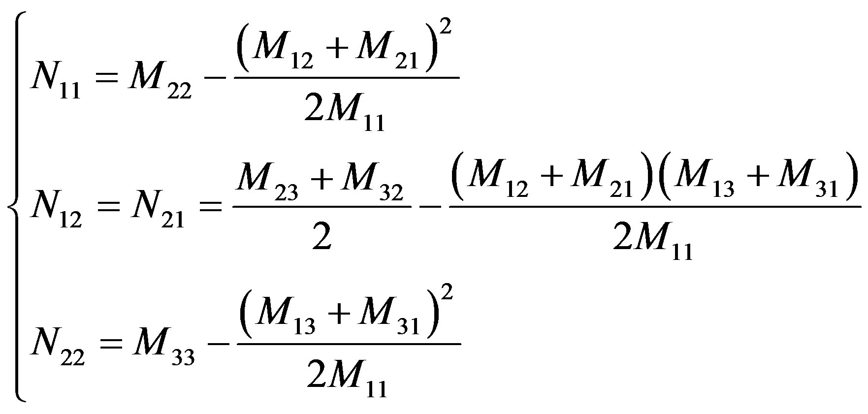
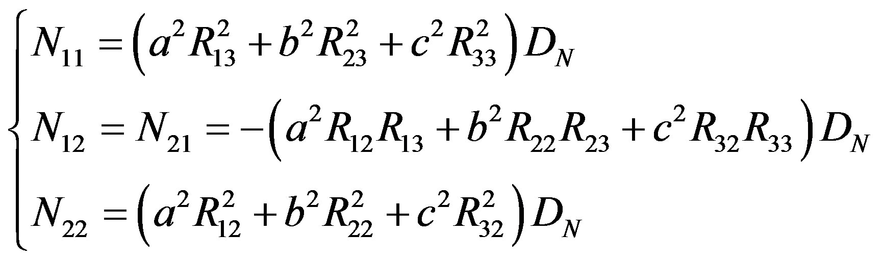
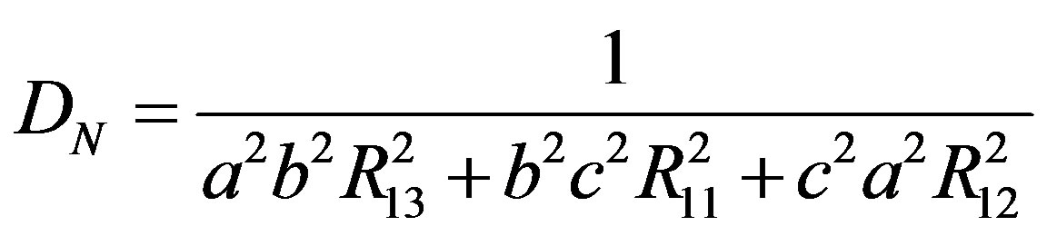
Above equations should be equal to Equation (20). Hence

(26)

Solving Equations (25) and (26), we have

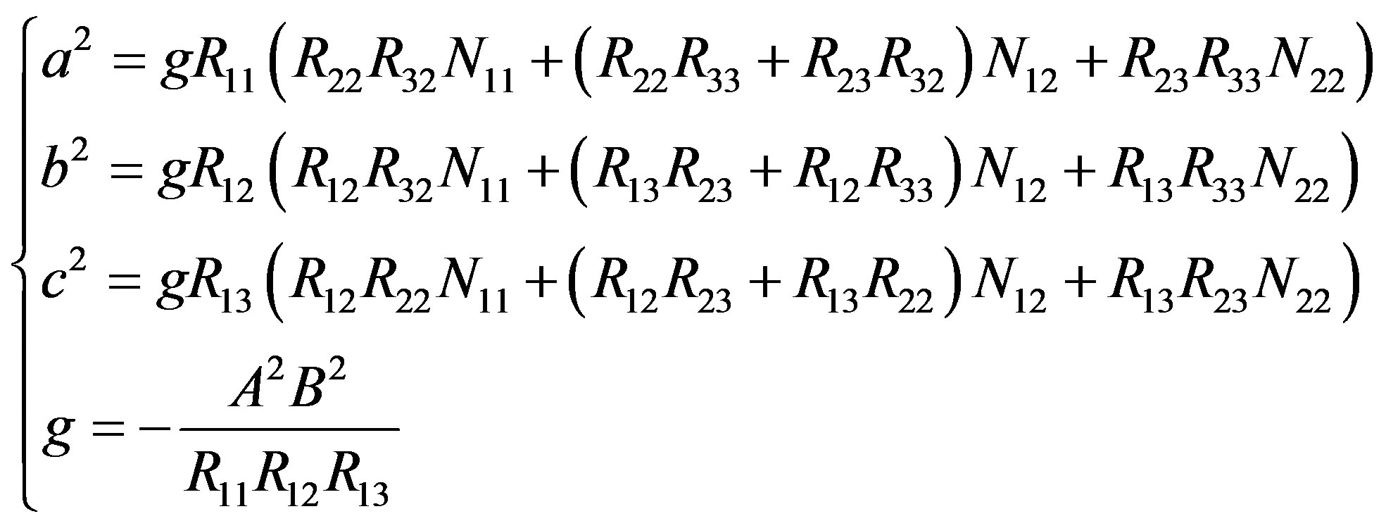(27)

where should be satisfied, otherwise there is no real solution. Since the process to solve the equations is long and complex, the Mathematica Ver. 5.1 is used for derivation.

If there is a formal solution of the three axes for the observed cross section and the supposed configuration, we test its propriety by reproducing lightcurves or other occultation cross sections. If a lightcurve of the asteroid around the occultation is obtained, we can determine its amplitude and phase at the time of occultation. Especially, a lightcurve phase at the occultation is significant in order to determine the sense of rotation, prograde or retrograde. If uncertainties in the observations of the occultation cross section and the lightcurve are small enough, we can determine a unique 3-D model of the asteroid by two cross sections and one lightcurve at an occultation. In the practical case, the propriety of the model is measured by the most likely method.

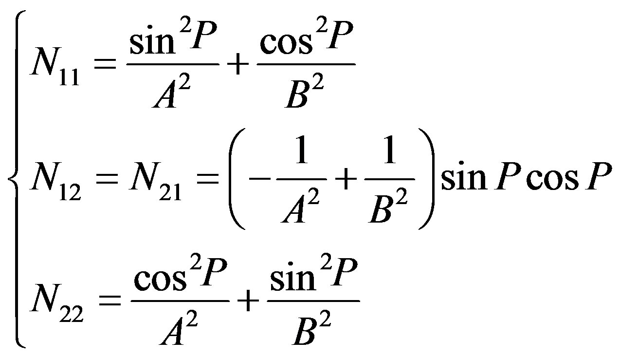
If a tri-axial ellipsoid model of the asteroid is assumed, the apparent ellipse of the cross section is given from Equation (18) with the components

(28)

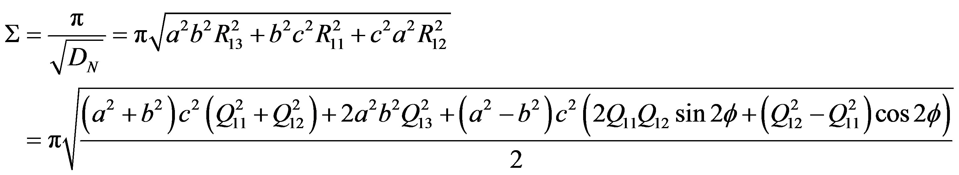
The eigenvalues of the coefficient matrix are given in Equation (23). The model amplitude of the lightcurve (derived from the cross section area) should be given by the square root of the ratio of the maximum and the minimum of the product of the two eigenvalues. The area of the cross section is derived from Equations (23) and (28)

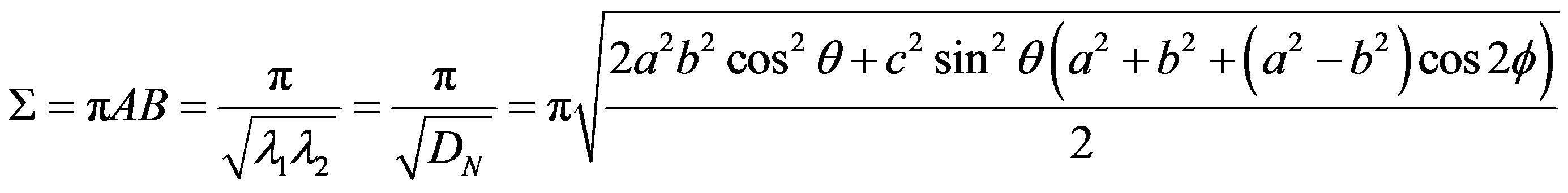(29)

The maximum and the minimum of are at and, respectively. Therefore the amplitude Δm is

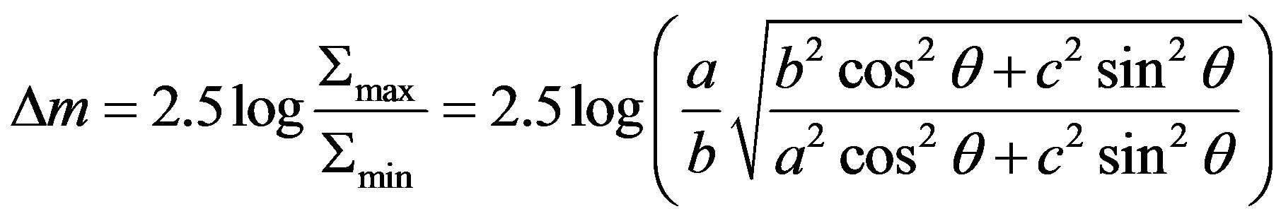(30)

Also, the phase angle at the minimum of the lightcurve is derived from Equations (11), (21), and (29),

(31)

Therefore depends on and. Hence the rotation phase angle at the lightcurve minimum is the derived from

(32)

Then we have

(33)

Therefore the lightcurve phase at the time of occultation measured from the minimum is related with the rotation phase angle by

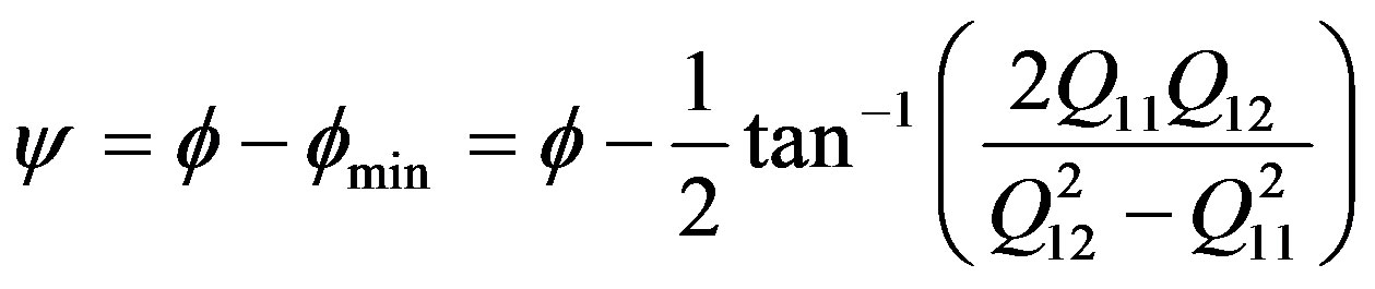(34)

Next, we evaluate the likelihood of the model. As stated at the beginning of this chapter, a configuration of an ellipsoid is described by seven parameters: the lengths of the three pricipal axes, the direction of the rotation axes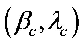, the rotation phase angle, and the rotation period. 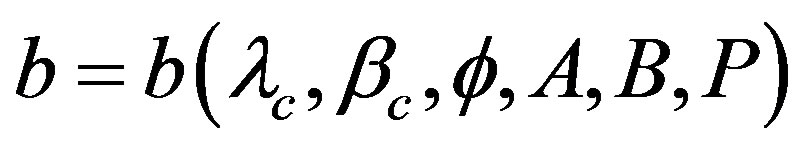On the other hand, we have some observed values of the lengths of the two principal axes of the apparent cross section, and the position angle of that for each occultation cross section. Also, we have some observed values of the lightcurve amplitude and/or the phase at the occultations. Then the fitness of an ellipsoid model is tested by how well the model can reproduce the observed cross sections and lightcurves. An indicator of the fitness is the likelihood.

First, if are supposed, one set of is determined uniquely from an occultation cross section by Equation (27). This is an initial ellipsoid model except for the rotation period p. Second, we test how well the ellipsoid model can reproduce other observed occultation cross sections and/or lightcurves. The likelihood about the lightcurve 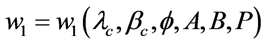and that about the cross section

are defined as follows,

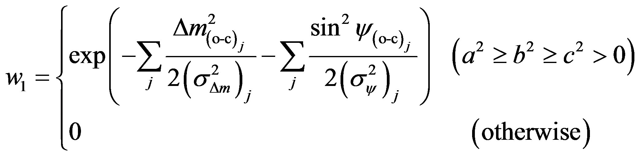(35)

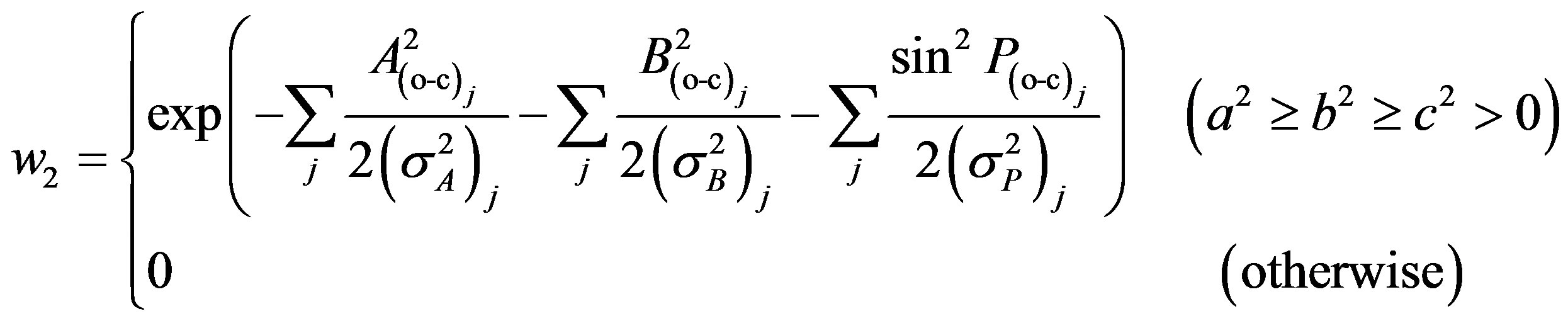(36)

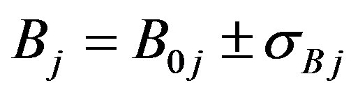
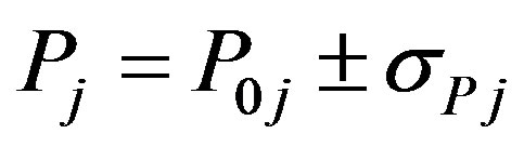
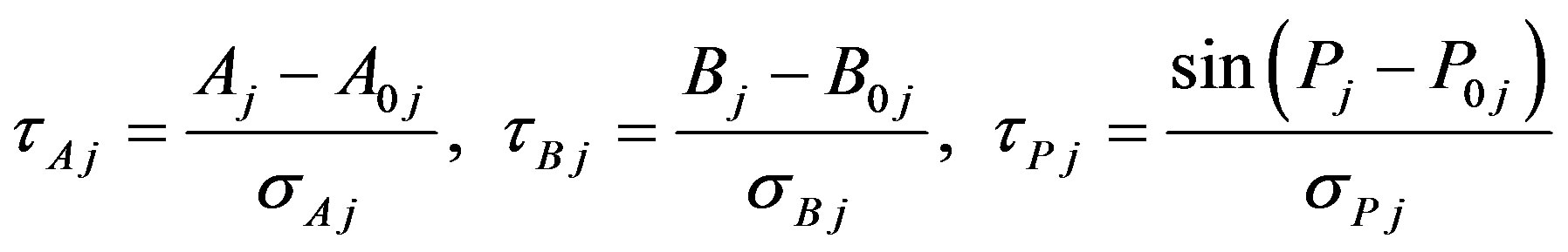
where the suffix “” indicates the difference of observed and calculated value of the j-th data, and, , , , are the standard deviations of each observed parameter value. Unless is satisfied, there is no solution.

Since the observed values have uncertainty, namely {, ,

}, total likelihood for a set of should be evaluated by a triple integration of these parameters using Gaussian weighting as follows,

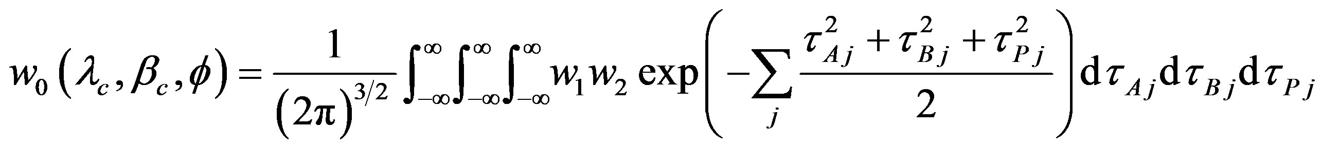(37)

where

(38)

Hence the likelihood is evaluated by the integral of on the rotation phase angle,

(39)

Result of above equations is shown in Figures 10-11.

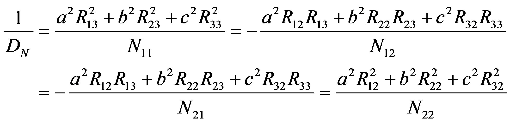
The probability distributions of the lengths of the three principal axes are derived similarly. From Equation (27), are functions of of an occultation cross section and supposed of a configuration of an ellipsoid model. Namely, 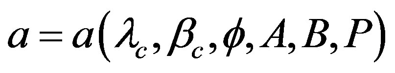, , and