International Journal of Astronomy and Astrophysics
Vol. 3 No. 2 (2013) , Article ID: 32738 , 8 pages DOI:10.4236/ijaa.2013.32017
An Intriguing Correlation between the Distribution of Star Multiples and Human Adults in Household
Hamaccabim St., Shoham, Israel
Email: alonretter@gmail.com
Copyright © 2013 Alon Retter. This is an open access article distributed under the Creative Commons Attribution License, which permits unrestricted use, distribution, and reproduction in any medium, provided the original work is properly cited.
Received January 17, 2013; revised February 20, 2013; accepted February 28, 2013
Keywords: Binaries; General; Surveys
ABSTRACT
It is a known fact that like people, some stars are singles, many others tend to couple in binaries, and fewer are in triples etc. The distribution of multiplicity in the 4559 brightest nearby stars was matched with that of human adults in household in six countries, in which this information could be dug and estimated. A strong resemblance between the two curves is evident. Monte Carlo simulations suggest that this result is significant at a confidence level higher than 98%. Apparently, there should be no connection between the two populations, thus this striking result may supply some clues about the way Nature works. It is noted that extended versions of this work were proposed three years ago, and two predictions of this absurd model have already been verified.
1. Introduction
Astronomy is the observational study of stars. Sociology is the scientific or systematic study of human societies. Evidently, there should not be any relation be tween the two fields. Yet, it is known that many stellar systems are coupled in binary stars [1] similar to people. Recent observational data of several thousand brightest nearby stars [2] and the following expert research analysis [3] supplied a unique opportunity for a comparison between the distributions of stellar and human multiples.
2. The Distribution of Stellar Multiples
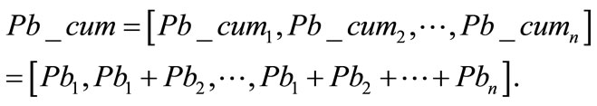
The multiplicities of stars were collected for a set of 4559 bright stars with Hipparcos [2]. The observed sample contained multiplicities up to 7. Taking into account the observational biases, it was concluded that the actual distribution of stars in 1, 2 ··· 7 multiples is respectively 1459, 2179, 517, 202, 101, 44, and 48 [3], which respectively are 32.1%, 47.9%, 11.4%, 4.4%, 2.2%, 1% and 1% of the total sample. Note that there were only 4550 stars in the simulated data. Table 1 lists these values and the mean number of stellar multiples, which is 2.04, as well as data up to multiplicity of 5 for American adults, which are described below.
3. The Distribution of American Adults in Household
The stellar multiplicity values were compared with human data—number of adults in household. The reasons for including only adults were discussed in preliminary papers [4,5]. It was argued that the distribution of stellar multiples should be matched with adults, and should not include children and old people. According to the perception of these papers, the total population—adults, children and elderly—should be compared with stars, planets and old stars such as white dwarfs and neutron stars. The distribution of multiplicity of this stellar population is, however, not known yet.
Data on Earth’s total population are not available, so single countries were examined. The distribution of multiple stars was initially compared with the 2009 data of USA adult population [6]. For family households the numbers of 1, 2 ··· 5+ members in the age interval of 18 - 65 years old in 1000 units are 14,900, 43,479, 9190, 2878 and 739. For non-family households the data (up to multiples of 7) are unfortunately given for all ages: 31,657, 5363, 821, 338, 99, 30 and 23 thousands. Therefore, we normalized these data by the ratio of adults (18 - 65 years old) to all population in non-family household, which is 26,712/38,331 ≈ 0.7, and estimated 22,061, 3737, 572, 236 and 106 thousands of 1, 2 ··· 5+ adults in this
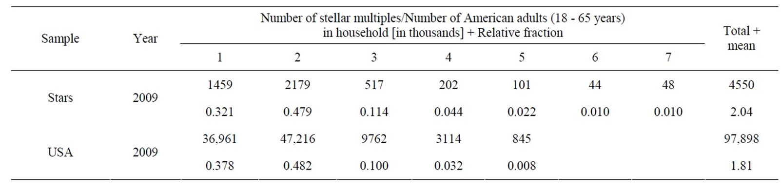
Table 1. Stellar multiplicity and number of American adults in household.
population. Adding together the values of family and non-family households, the final numbers of 1, 2 ··· 5+ adults in the age interval of 18 - 65 years old in 1000 units in all population are 36,961, 47,216, 9762, 3114 and 845. These data correspond to 37.8%, 48.2%, 10.0%, 3.2% and 0.8% of 1, 2 ··· 5+ adults in household. The American adult data are shown in the last entry in Table 1. The mean value is about 1.81 adults per household, which is close to the average stellar multiplicity –2.04.
In Figure 1 we plot the two distributions as well as a third dataset which is discussed below. The resemblance between them is outstanding. Indeed, we estimated from extensive Monte Carlo simulations that the distributions of stars multiples and American adults in household are consistent with each other with a probability level higher than 98% (Appendix). Note that previous works [4,5,7] ignored the contribution of non-family households to the adults population. In this case the match between the two curves was less prominent, and the significance level was slightly lower, but the mean number of adults in household was closer to the average stellar multiplicity value.
4. The Distribution of Persons in Household in Several Countries
Following the referee’s request, data on other countries were studied. We searched for information on the distribution of adults in the national statistical bureaus of the ten most populated countries [8]. Relevant data were only found in USA, in which the details of the statistics were the most comprehensive. In the other cases either no data were found or some partial data with no age information were available. An email was sent to the statistical bureau of each country requesting for the required data, but either no response was received or the reply was not helpful. The sample was thus increased to include a few more cases. English speaking countries were chosen to avoid language problems. An exception is Israel, the native country of the author. Table 2 summarizes the data search.
USA was the only country in the sample in which data on the number of persons in household were given with respect to age groups. Thus, it was decided to collect data
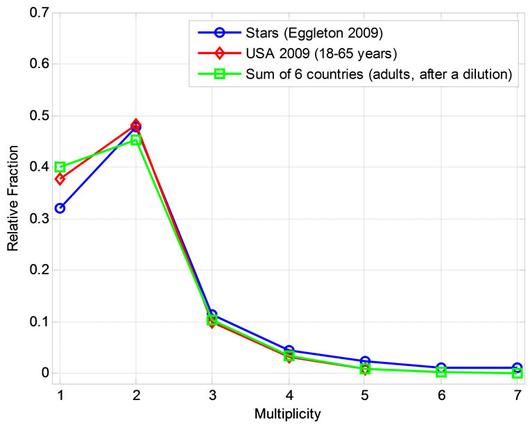
Figure 1. A comparison between the distributions of star multiples (blue circles), American adults in households in 2009 (red triangulars), and adults (concluded by a dilution) in the sum of six countries (green squares). There is a remarkable similarity between the stellar curve and the human distributions. Numerical simulations suggest that these results are highly significant.
on the total number of persons in household bearing in mind that this is not the optimal parameter for the comparison. Relevant data were collected for five more countries—Japan, UK, South Africa, Canada and Israel.
Table 3 comprises the data in the countries in which they were accessible. It lists the number of 1, 2 ··· 7+ persons in household as well as fraction from the total population and the total and mean number of persons in household. For UK and Canada the figures are only given up to 6+ persons in household. Note that the average values may be slightly larger than the mathematical calculation due to possible higher multiplicities. The sum of all six countries is also shown as well as the mean distributions of these countries, which actually assigns an equal weight to every single country. Finally, an artificial dilution of the sum and mean distributions to adults is calculated (see below).
It is noted that there was an attempt to collect data around the year 2009—the time of the astronomical data. The reason for this is elaborated in the discussion. There

Table 2. Results of data search in ten most populated countries + six more.
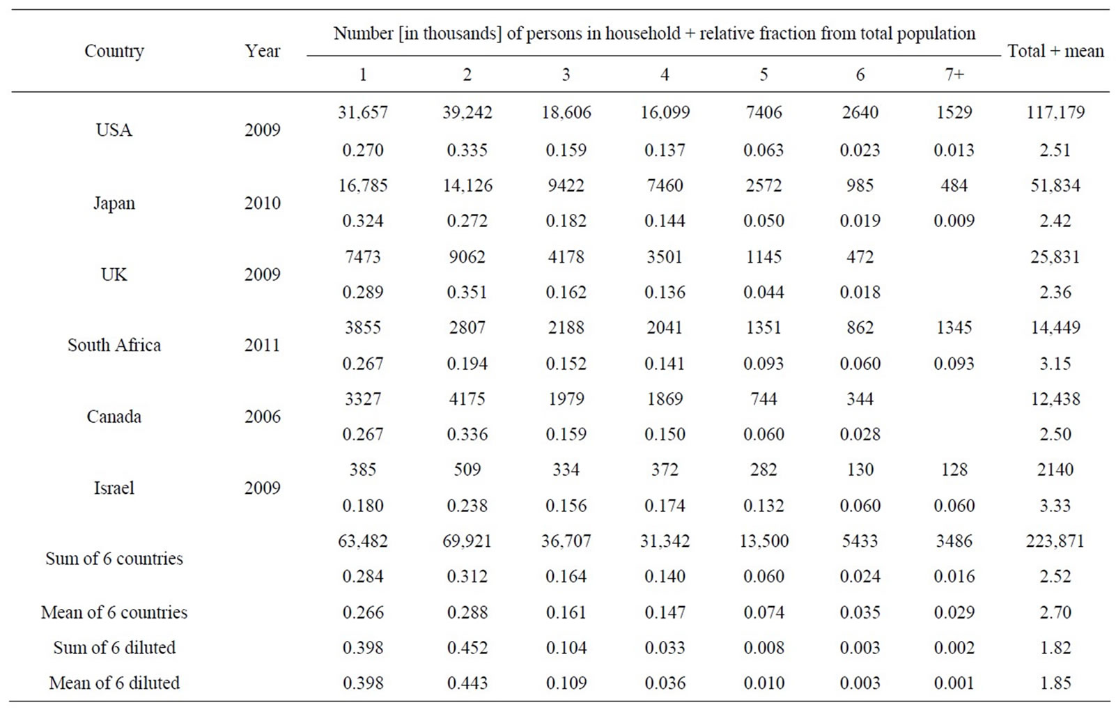
Table 3. Number of persons in household in countries in which useful data were available and fraction relative to the total population. The last four entries present the sum and mean of the six countries, and their distributions after a synthetic dilution of the population to ages 18 - 65 years. See text for details.
are, however, minor differences between relative values (in percentages) from various years, and data are available only during the last few years or decades at max. We also comment that for all countries in the sample the total number of persons in household in Table 3 is lower than the overall population values in Table 2. The most likely reason is that the censuses are partial.
Figure 2 displays the distributions of number of all persons in household in the countries in which data were available. There is obviously some variety between different countries. The distributions of USA, UK, Canada and Israel are quite similar with a peak at 2. The curves of Japan and South Africa are not far from it with the highest peak at 1 person per household. The dotted-dashed line in red displays the distribution of the sum of the six countries, which also peaks at 2.
5. Diluting the Distribution of All Persons to Adults
As noted above, we believe that the correct comparison between stellar multiples and humans should be to number of adults in household rather to all people. Thus, we attempt deriving this distribution by subtracting children and elderly from the total population. The ratios between American adults (18 - 65 years) to all people in family household in the cells 1, 2 ··· 5 are: 1.398, 1.441, 0.628, 0.232 and 0.131. For bins 6 and 7, no data are available. To be consistent with the decreasing trend from cell 2 to 5, we assumed factors of 0.5 and 0.25 between these cells and bin 5. Note that the values in the last two cells are relatively small and have a minor effect on the distribution. The distribution of adults was then calculated, normalized to one, and tabulated at the bottom of Table 3. The dilution impact was some shift towards lower num-

Figure 2. The distributions of number of all persons in household in different countries. The dotted-dashed line in red displays the sum of the six countries. Note that the Canadian data cover the USA values, which are almost identical to them.
bers. Figure 3 displays this effect for both the sums and means of the six countries. The distribution of all persons in the sum of the six countries, which was displayed in Figure 2 as well, is shown in red, while the green curve presents the synthetic distribution of adults (18 - 65 years) in this sample. The distribution of the mean of the six countries is shown in blue together with the one standard deviation (1σ) errors. The diluted distribution of the means (in black) is very like the diluted distribution of the sums. The diluted distribution of the sum of the six countries is also plotted in Figure 1. A remarkable similarity between this distribution and that of stellar multiples is seen. It was deduced from Monte Carlo simulations that the two distributions are consistent with each other with a probability level higher than 99% (Appendix).
6. Discussion
The results presented in this paper are quite strange, extraordinary and difficult to believe and to understand. This work presents a fantastic numeric resemblance between the distributions of stellar multiples observed in the night skies and humans. From extensive numerical simulations it was concluded that the similarity between number of American adults in household and stars multiplicity is significant at a confidence level higher than 98%. Furthermore, the distribution of stellar multiples is also consistent with the synthetic distribution of adults in the six countries at a confidence level higher than 99% (Appendix).
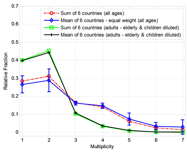
Figure 3. The distribution of number of all persons in households in the sum (red circles) and mean (blue diamonds) of the six countries. The vertical bars represent 1σ errors of the means. The synthetic distributions of the sums (green squares) and means (black pluses) for adults after the subtraction of children and old people using the American coefficients are also shown. See text for further details.
There is still a little chance that the similarity between human adults and stars is only a coincidence. The data used in this work were taken from partial samples. The distribution of star multiples was built using observational data of the 4559 brightest nearby stars and a theoretical analysis of the observational biases, which may suffer from some uncertainties. The collection of data on persons in household suffers from a bias of English speaking countries. In addition, the distribution of adults in household in USA and in the sum of the six countries was estimated using simplified coefficients taken from USA data. All these facts naturally lead to some uncertainties. Yet, to date, these samples are the best available.
The sum of adults in the six countries is strongly influenced by a single country—USA, whose data constitutes about a half of the total population. Note, however, that if all countries are given the same weight, the results and significance level are hardly affected as the distribution of the mean values of the six countries is almost identical to the distribution of the sum of all data (Table 3, last 4 entries, Figure 3, see also Appendix and Table 4).
The distributions of stellar multiples and adults in household are not simple Gaussians so they are not common. It can neither be argued that there is a general Nature rule that states that individuals tend to couple in a certain way with a peak at two because it is clear that the multiplicity distributions of certain animal species (e.g. fish or bees) are clearly different. It seems that the surprising resemblance between the distributions of stellar multiples and human adults requires some explanation.
The perception that led to this research is similar to one interesting interpretation of Quantum Mechanics that seems absurd—that the observer influences the experiment. The educated reader may ask: “Why comparing the current distribution of humans with that of stars, which is older by the time interval, it took light to reach Earth?”
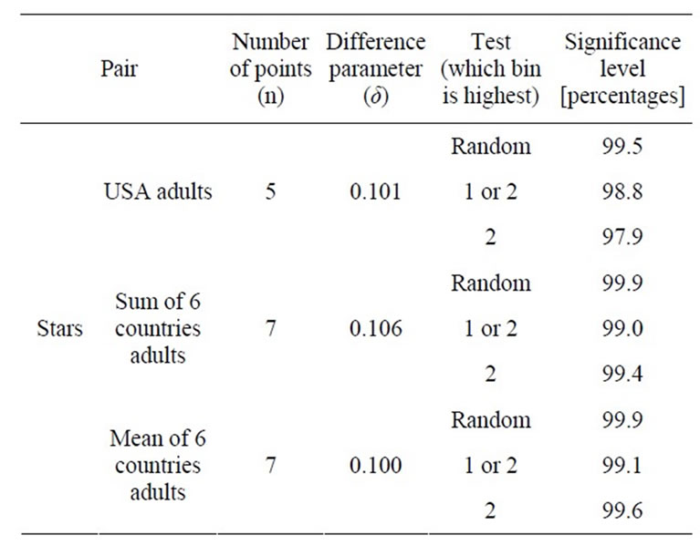
Table 4. Different tests and the resulting significance levels.
According to this perception, the results depend on the time of the observations. Thus, we expect that people with a different distribution, who observe the universe in the future with better equipment, would reach different conclusions! This is the reason for trying to collect data around the same time (Sections 2-4, Tables 1 and 3).
Finally, this paper actually presents only a glimpse of our ideas, which we admit sounds completely absurd. Some similarity between the distributions of American children and planets was found as well, although for a small sample of planets [4,5]. Combining this result with the significance value of 98% estimated for the resemblance between stellar multiples and American adults in household (Appendix), the significance level is even higher and cannot be regarded as an anecdote. These results should be re-examined in the future when larger data samples are available, but the picture that arises from them [see also 24] is quite strange. It is noted that two predictions of the Astro-Sociology model [4,5] for orphan and adopted planets have already been verified by observations [25] and simulations [26,27]. This fact adds some support to this unusual perception. It is also anticipated that many more predictions of the theory, in example for twin planets, will be confirmed within the next few years.
7. Acknowledgements
It is a pleasure to thank Shlomo Heller (Kartar) for many stimulating discussions, the anonymous referee and Ram Krips for valuable comments and Doron Retter for some help preparing the tables.
REFERENCES
- B. Warner, “Cataclysmic Variable Stars,” Cambridge University Press, Cambridge, 1995. doi:10.1017/CBO9780511586491
- P. P. Eggleton and A. A. Tokovinin, “A Catalogue of Multiplicity among Bright Stellar Systems,” Monthly Notices of the Royal Astronomical Society, Vol. 389, No. 2, 2008, pp. 869-879. doi:10.1111/j.1365-2966.2008.13596.x
- P. P. Eggleton, “Towards Multiple-Star Population Synthesis,” Monthly Notices of the Royal Astronomical Society, Vol. 399, No. 3, 2009, pp. 1471-1481. doi:10.1111/j.1365-2966.2009.15372.x
- A. Retter, “The Meaning of the Singularity: 2. Astro-Sociology: Predicting the Presence of Twin Planets (Short Version),” 2010. http://vixra.org/abs/1004.0129
- A. Retter, “The Meaning of the Singularity: 2. Astro-Sociology: Predicting the Presence of Twin Planets (Extended Version),” 2010. http://vixra.org/abs/1004.0130
- US Census Bureau, “tab-F1-all_2009, tab-H2-all_2009,” 2013. http://www.census.gov
- A. Retter, “An Intriguing Correlation between the Distribution of Star Multiples and American Adults,” 2011. http://vixra.org/abs/1107.0051
- Worldatlas, “Countries of the World,” 2013. http://www.worldatlas.com/aatlas/populations/ctypopls.htm
- National Bureau of Statistics of China, 2013. http://www.stats.gov.cn/english/
- Ministry of Statistic and Program Implementation, 2013. http://mospi.nic.in
- Indonesian Bureau of Statistics, 2013. http://www.bps.go.id
- Brazilian Institute of Geography and Statistics, 2013. http://www.ibge.gov.br/english
- Pakistan Bureau of Statistics, 2013. http://www.pbs.gov.pk
- Bangladesh Bureau of Statistics, 2013. http://www.bbs.gov.bd/home.aspx
- National Bureau of Statistics, 2013. http://www.nigerianstat.gov.ng
- Federal State Statistic Service, 2013. http://www.gks.ru/wps/wcm/connect/rosstat/rosstatsite.eng
- Statistics Bureau, y0216000, 2013. http://www.stat.go.jp/english/index.htm
- The Office for National Statistics, 2013. familieshouseholds_tcm77-284827, http://www.ons.gov.uk
- Statistics South Africa, 2013. http://www.statssa.gov.za/
- Statistics Canada, 2013. http://www.statcan.gc.ca
- Australian Bureau of Statistics, 2013. www.abs.gov.au
- Central Bureau of Statistics, 2013. http://www1.cbs.gov.il
- Statistics New Zealand, 2013. http://www.stats.govt.nz/
- A. Retter and S. Heller, “The Meaning of the Singularity: 1. A Single Particle Universe,” 2010. http://vixra.org/abs/1004.0128
- T. Sumi, et al., “Unbound or Distant Planetary Mass Population Detected by Gravitational Microlensing,” Nature, Vol. 473, No. 7347, 2011, pp. 349-352. doi:10.1038/nature10092
- H. B. Perets and M. B. N. Kouwenhoven, “On the Origin of Planets at Very Wide Orbits from the Recapture of Free Floating Planets,” Astrophysical Journal, Vol. 750, No. 1, 2012, Article ID: 83. doi:10.1088/0004-637X/750/1/83
- K. M. Kratter and H. B. Perets, “Star Hoppers: Planet Instability and Capture in Evolving Binary Systems,” Astrophysical Journal, Vol. 753, No. 1, 2012, Article ID: 91. doi:10.1088/0004-637X/753/1/91
- W. H. Press, S. A. Teukolsky, W. T. Vetterling and B.P. Flannery, “Numerical Recipes,” Cambridge University Press, Cambridge, 1992.
Appendix—Significance Estimates
The distributions of people and stars multiplicity were discussed above and it was concluded that they are alike (Figure 1). The purpose of this appendix is to check whether these results are significant. One may try to use the Kolmogorov-Smirnov (KS) probability test [28] to check whether two different distributions are consistent with each other. This test is, however, adequate for a large number of points that can get continuous values, while the relevant distributions of stars and adults only have a few discrete points. Therefore, it was decided to test the statistical significance of the results by extensive Monte Carlo simulations.
Given a distribution,  for bins
  that complies
  for
for  , we posed the question: “what is the chance probability to obtain by random a second vector distribution,
  with
with ?” We defined a difference parameter
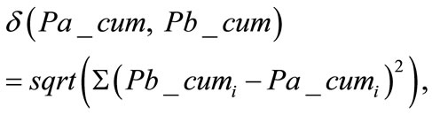
between the corresponding cumulative distributions:

For the cumulative distributions of the pair—American adults ([0.378, 0.860, 0.960, 0.992, 1]) and stars ([0.321, 0.800, 0.914, 0.958, 1]), n = 5 and δ = 0.101. Note that the stars data were re-arranged into 5 bins in order to fit the first data set. For the synthetic cumulative distribution of adults in the sum of the six countries ([0.398, 0.850, 0.954, 0.987, 0.995, 0.998, 1]), and stars ([0.321, 0.800, 0.914, 0.958, 0.980, 0.990, 1]), n = 7 and δ = 0.106. The third pair was the cumulative distribution of adults in the mean of the six countries ([0.398, 0.841, 0.950, 0.986, 0.996, 0.999, 1]), and stars. For this couple δ = 0.100.
For the test we built one million random distribution samples with noise taken from the data using a few different methods. First, the mean and standard error of the Pa data were found, and then for every simulation we raffled Gaussian distributed noise and obtained n random numbers around the data mean. Negative numbers were shifted upwards and given a random number around 0.01, and the total simulation vector was normalized to 1, so . From this initial simulated vector,
  , the cumulative distribution was calculated to obtain the final probability vector

The difference parameter between this simulated distribution and the second given distribution, δ (Ps_cum, Pb_cum), was calculated. For one million simulations, one million values of this parameter were obtained. The significance level was defined as the ratio between the number of values higher than the observed difference parameter, δ (Pa_cum, Pb_cum), calculated above, to the total simulations number. This test suggested that there is 99.5% chance probability that the first pair (American adults, stars) is significant and 99.9% for the second (adults in the sum of the six countries, stars) and third couple (adults in the mean of the six countries, stars).
The strongest peak in the distributions is at the second cell (2) and the second highest is at bin 1. We repeated the simulations, giving a preference for the largest probability value in each simulation to be either at bin 1 or 2, while all other n-1 figures were randomly shuffled in the remaining bins. The results of these simulations were that there is 98.8% chance probability that the two distributions of stars and American adults are consistent with each other. For the second and third pairs: stars— adults in the sum or mean of six countries values of 99.0% and 99.1% were found. These figures were adopted in the paper and they mean that the couples are highly significant. This is a conservative approach, because a priori given the distribution of adults, the distribution of stars could be completely different, say with all multiples above n = 5, and there is no reason why the strongest peak in the astronomical distribution would be either at 1 or 2.
We performed another test that clearly underestimated the significance level of the results. We imposed the highest probability value in the simulated vector exactly as observed—in the second bin. The other values were randomly placed in the other bins. In this test the resulting significance level was 97.9% for the first couple, 99.4% for the second and 99.6% for the third. These simulations confirmed that once the distribution of adults is given, there is a very low chance probability to randomly obtain the observed distribution of stars. Table 4 summarizes the results of the significance tests.
The data and errors were also modeled in a different way. We either fitted a 2D or 3D polynomial to the data. The standard errors were calculated from the difference between the fit and the data. Then we raffled random numbers according to the standard error and added them to the fit to obtain n random numbers. Negative values were given random numbers around 0.01, and the total simulation vector was normalized to 1. The data bins were either randomly shuffled or given some preference in the first two bins or only in the second cell as discussed above. The cumulative distribution was then calculated to obtain the final simulation vector, and the difference parameters, δ (Ps_cum, Pb_cum), was calculated. The outcome of these simulations was very similar to the results obtained above with differences of up to tenths percent between the two methods.