ABSTRACT

The exploitation of an oil field is a complex and multidisciplinary task, which demands a lot of prior knowledge, time, and money. A good reservoir characterization is deemed essential in the accomplishment of Enhanced Oil Recovery (EOR) pro- cesses in order to estimate accurately the properties of the porous medium affecting the flow properties. Several techniques at a field scale are currently being used to determine these properties, which are time and money consuming. But these alone do not guarantee the success of the project. Reservoir simulation and numerical techniques were then included in the pre-development and follow-up studies as an effective tool to determine the productivity and future behavior of the oil field. As the computational power increased, more advanced and detailed models were developed, including different chemical and physical phenomena. But alongside this process, there was an active research in the area of reservoir simulation, improving the accuracy and efficiency of the numerical schemes used for the flow, transport, and energy equations. The aim of this review is to address the topics described. Firstly, the origin of an oil recovery process, the economic factors and field tests involved are introduced. Secondly, the oil and porous medium origin and characterization as well as an introduction to the fundamental concepts and equations are associated to reservoir simulation. Finally, a brief description and analysis of the techniques are used in reservoir simulation employing finite difference methods, their downsides and possible ways to overcome these problems.

Keywords:

Petroleum Engineering, Enhanced Oil Recovery, Reservoir Simulation, Numerical Analysis

1. Oil Origin and Formation

1.1. Introduction

The era of discovery and subsequent exploitation of the denominated “easy oil” (part of the so called conventional reserves) is over [1] - [5] . After primary and secondary recovery, oil companies have begun with more complex Enhanced Oil Recovery (EOR) processes involving fluids or chemical reactions that require a greater detail of the phenomena taking place in the porous medium. In addition to these complications there exist non-technical related factors that might increase the risk of an investment [6] . An example of this may be the development of off-shore platforms, plants located in remote areas of the world or the exploitation of unconventional deposits (heavy oil, shale oil, tar sands). All these projects require a prior investment (in the order of several tens of millions of dollars high risk projects), so companies make use of several techniques in the stage of feasibility analysis to limit this risk and increase the chances of success of the operation (Figure 1) [7] [8] .

These techniques, used to predict and optimize the exploitation, include laboratory and field tests (e.g. seismic 2D/3D/4C before starting operations and 4D to follow up the changes during exploitation, geostatistics) to give an idea of the conditions of the porous medium and its production performance [9] - [13] . However, these tools have proven to be insufficient [12] [14] [15] and therefore oil companies have begun using computational tools to predict and optimize their projects and production facilities, which is known as Reservoir Simulation. The latter consists in solving numerically the differential equations describing the fluid flow in porous media, which have no analytical solution, taking into account all geological, physical, chemical and/or mechanical

phenomena occurring during operation so as to analyze and predict behavior as a function of time. The reservoir simulation can be used as well in inverse engineering problems for optimizing existing numerical models and couple the dynamic/historic data (production) in the simulation [15] - [18] .

Generally speaking, reservoir simulation consists of three main parts: the physical characterization of a geological model describing the rock formation; a model characterizing the fluid flow and finally “well models” which describe the conditions under which fluids are injected or extracted from the reservoir [19] . The latter, along with the wellbore and the primary surface facilities, constitutes what is known as upstream. During the last 30 years numerous theoretical and practical advances have been developed due to the appearance of new numerical techniques and increased computational power, respectively [15] [20] . This led to a new generation of more complex and detailed models. The accurate representation of the reservoir and the fluid contained in it is an issue that still needs to be more carefully addressed in order to reduce risks in exploration and production (E&P) projects. One of the most important points is related to the scales of the models: current grids are still large when compared to the geological characterization, description of chemical processes or fluid flow. Most of current numerical models used in reservoir simulation may contain from 10⁵ to 10⁸ grid blocks, depending on the model type, complexity, computational power available and fluid behavior.

The development of increasingly complex and detailed models requires the use of numerical techniques to solve these at reasonable times. Moreover, the representation of the properties of the porous medium and the characteristics of crude oil and natural gas at high pressures and temperatures may differ from laboratory tests, causing differences between the results and simulation. Another important topic is how to assess and properly estimate the properties of the rock formation. Geologists use statistical techniques in order to recreate the model properties of a porous medium, which are determined by several tests (e.g. seismic studies, drill core samples and even production data). However, other numerical tools are required (e.g. Monte-Carlo or Stochastic Processes) to take into account the effects of uncertainties in the model [21] [22] .

The aim of this review is to briefly describe the characterization of porous media and its main parameters. Then, models governing fluid flow in porous media are introduced. This consists in Darcy’s equation and the more complex compositional model for multiphase flow (where the component transfer between phases introduces nonlinearities in the mass transport equation), which is useful to describe chemical EOR operations. The second part comprises a brief explanation of the numerical methods used as well as the problems associated with these schemes (numerical dispersion and dissipation), and possible solutions using advanced numerical schemes.

1.2. Origin of the Oil

A reservoir is an underground trap where different fluids (water, oil and gas) have accumulated due to a migration from the source rock where they were originated. The porous medium is generally considered of sedimentary origin and consists of a series of microchannels (about 1 - 100 microns diameter) interconnected where these fluids can flow (Figure 2). These formations may have some tens of meters thickness, but may extend several kilometers in the lateral directions [23] .

The origin of crude oil prior to the migration and deposit of hydrocarbons in the porous media is also a long and complex process [25] - [27] . The source of hydrocarbons consists of a series of phenomena, both organic and inorganic, taking place during long periods of time (in the order of million years) [28] . Most of these hydrocarbons originate in organic decomposition processes. The first stage (called diagenesis) involves the sedimentation of remains of dead plants and animals. Under these conditions, at low depths, the action of bacteria produce methane, water and CO₂, leaving as reaction products of kerogen substances (cyclic and large hydrocarbon molecules containing oxygen, nitrogen and sulfur). The second process, called catagenesis, occurs at greater depths and temperatures. In this region, known as the oil window zone, the kerogen molecules break in smaller, heavy hydrocarbons forming the oil phase. At higher temperatures the cracking of hydrocarbons continues creating lighter compounds, first wet gas and subsequently dry gas. Finally, at even greater depths, the last process takes place (called metagenesis), where the remaining kerogen is out of hydrocarbons and subsequent cracking processes terminate when there is no hydrogen in the compound. The result of these reactions is the formation of graphite (Figure 3).

1.3. Porosity and Permeability

A porous rock formation is composed of a solid part, called solid matrix, and the remaining void space or microchannels whereto oil migrates [31] . The volumetric fraction of these channels is denominated porosity of the porous media. The latter depends on the fluid pressure, if the rock is compressible, or in some other phenomena which may take place (e.g. adsorption of chemical components during EOR processes). The following list provides typical values of porosity according to the origin of the rock formation [32] [33] : Consolidated sandstones 0.05 to 0.3; limestones 0.1 to 0.4; uniform spheres with minimal porosity packing 0.25; uniform spheres with normal packing

0.35; unconsolidated sands with normal packing 0.40 and unconsolidated clays 0.60.

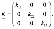
The permeability of the formation is a property that characterizes the ease with which fluids can flow when a pressure gradient is applied between two points. Nonetheless, reservoir rocks usually have no uniformity in their properties because of the mechanisms involved on its formation, thus the permeability will have a large dispersity in its values [34] [35] . The fluids used commonly in EOR operations, more mobile than oil, occupy the high-permeability zones (e.g. faults or fractures), with the result that large areas of oil will be bypassed, reducing the efficiency of the process. Mathematically, the permeability can be expressed as a diagonal tensor (K). When the medium is isotropic then the permeability can be represented as a scalar function. Due to transitions between different rock types, the permeability may vary swiftly throughout the reservoir, going from extreme low permeability areas of 1 mD to areas with permeabilities exceeding 10 D.

In order to develop a mathematical model of the porous medium, Corey [32] established several restrictions: the whole void space of the porous medium is interconnected; the mean free path length of the fluid molecules or molecules contained in the fluid must be negligible when compared to the dimensions of the pore channels, and the dimensions of the void space must be small enough so that the fluid flow is controlled by adhesive forces at fluid-solid interfaces and cohesive forces at fluid-fluid interfaces (in multiphase systems) [31] . These assumptions allow excluding any disconnected channels in which there can be no fluid flow, eliminating the difference between the concepts of total porosity and effective porosity. Furthermore, since the dimensions of the molecules or particles in the fluid are negligible with respect to the microchannels, a suitable replacement for a hypothetical continuous medium can be performed. Finally, considering the microscopic size of the channels allows taking into account physical phenomena that in other cases would be negligible. In order to derive a mathematical model at the macroscopic level, each point in the continuum is assigned average values over representative elementary volumes of the quantities at the microscopic level. The advantage of this technique is that leads to a set of macroscopic equations that do not need an exact description of the microscopic configuration, as it would be the case with Navier-Stokes equations [31] .

1.4. Representative Elementary Volume

The flow of reservoir fluids in porous media can be described at several different scales, from a microscopic to a macroscopic/formation scale. In order to perform large-scale reservoir simulations, a microscopic description of the flow channels would be too demanding for the computational power available and besides to characterize a reservoir rock so accurately to determine the geometry of the pore network is beyond the scope of modern techniques and equipment. A continuum scale description is then utilized, and its behavior is governed by forces acting between the different fluids and the rock formation. The goal of a reservoir continuum model is then to average both the fluids and reservoir rock [28] [36] - [39] . In order to develop the mathematical model based on a continuum, the concept of Representative Elementary Volume (REV) (Figure 4) is introduced. This is based on the hypothesis that certain properties of both the fluid and the rock may be considered constant along a certain range of scale and thus it establishes limits for the physical scales in the numerical models. If a REV cannot be identified for a specific porous medium then this concept cannot be applied and the macroscopic approach should be discarded [40] .

The procedure for estimating REV dimensions and establish boundaries between microscopic and macroscopic scales is explained below using the porosity in Figure 4 as an example [31] . A porous medium is then considered occupying the domain Ω, with a volume V(Ω). A subdomain Ω₀(d) Ì Ω with a characteristic dimension d is also defined. Furthermore, the porosity piece-wise function is defined in Equation (1) as follows,

(1)

Then, the porosity of an element with characteristic dimension d is defined by Equation (2),

(2)

This relationship allows explaining the evaluation of the porosity as a function of the dimension d. For sizes smaller to a value d_m the porosity varies significantly, with no particular pattern or trend; then, if the value of said dimension is between d_m and d_M, the value of the porosity plateaus and remains constant for the entire considered range. Finally, for values greater than d_M, the porosity may remain constant in the case of a homogeneous medium, while in the case of an heterogeneous one, the function becomes again chaotic [41] [42] . The volume with dimensions between d_m and d_M is called a representative elementary volume (REV) (Figure 4).

2. Fluid Flow Models

In underground processes in porous media, fluid flow involves mainly convection (advection and diffusion) of the different phases through a heterogeneous medium. The equations used to describe the flow at a microscopic level or poralscale are variations of Navier-Stokes (creeping flow) and the mass conservation law. At a macroscopic level, Darcy’s law [43] was derived and it is used to describe flow behavior. Also, the effects of the displacing process on the rock formation will be considered negligible even though these mechanisms are sometimes necessary to repre- sent first-order effects (e.g. adsorption) [44] [45] . When dealing with multiphase/ multicomponent flows, some of the processes therein involved are characterized by the chemical and physical interaction among the components present in the fluids. Therefore, diffusive and/or dispersive mixing of these components is often critical and must be correctly understood and modeled in order to obtain accurate results. Molecular diffusion is typically quite small in porous media processes. Nevertheless, hydrodynamic dispersion may be important and therefore it should be incorporated in the flow equations. This can be done by means of the standard diffusion/dispersion tensor [46] [47] , provided that the degree of the heterogeneity is not too large (Dykstra-Parsons coefficient < 0.50) resulting in a Fickian behavior. However, when the permeability variations are large a non-Fickian behavior was reported (anomalous dispersion) [48] - [52] .

Generally, three fluid phases may exist inside a reservoir (Figure 2): aqueous/ brine (the phase containing predominantly water), oleous (the phase containing liquid hydrocarbons) and gas phase, which contains lighter gaseous hydrocarbons (Figure 3). In the case of single phase systems, the void space of the porous medium is filled by a single fluid or by several fluids completely miscible with each other. In multiphase systems the void space is filled by two or more fluids that are immiscible with each other, thus maintaining a distinct boundary between them. Formally speaking, the solid matrix of the porous medium can also be considered as a phase called the solid phase. Each phase may also be composed by many chemical components. For example, oil is a very complex mixture of hundreds of hydrocarbons with different chemical properties. In order to derive a set of equations for the fluid flow some terms should be defined beforehand. Firstly, the term phase stands for matter that has a homogeneous chemical composition and physical state of a system under consideration that is separated from other such portions by a definite physical boundary. Secondly, it is defined as component present in a phase to the matter that is composed of an identifiable homogeneous unique chemical species or of an assembly of species [41] . The number of components needed to describe a phase is given by the conceptual model, i.e. it depends on the physical processes to be modeled and the desired accuracy. In many oil reservoirs (above bubble point pressure) crude oil contains some amount of dissolved gas. It is acceptable to assume that the oil and gas compositions are fixed [15] [20] [26] , and that the solubility of the gas in the oil depends on pressure only. Provided these conditions are met, then it is possible to consider the pseudo-components oil and gas.

Both microscopic and macroscopic effects control the movement of fluids in the reservoir. At the pore scale, interfacial tension (IFT) and capillary effects control the fluid behavior. Macroscopically, fluid flow is controlled by reservoir heterogeneity and mobility differences between the fluids. Viscosities, capillary pressure, IFT and mobility differences vary throughout the reservoir and depend mainly on phase saturations, their interactions and molecular compositions. Chemical components may transfer between contacting phases, altering the fluid properties of both. Interactions between the fluids or their components and the reservoir rock may also impact performance (e.g. adsorption of chemical components onto the surface of the rock altering the wettability). Thermal effects are generally very small due to the large heat capacity of the rock. However, in EOR thermal processes (steam flooding or in-situ combustion), the conservation of energy in the REV should be considered.

2.1. Single Phase Flow

The governing equations for single phase flow in porous media are the conservation of mass, the Darcy equation and an equation of state (EOS). Considering the flow of a single fluid with density ρ through a REV of a porous medium the differential form of the continuity Equation (3) can be expressed as [15] [19] [20] [34] [36] [53] - [55] ,

(3)

where f is the porosity of the rock formation, q represents the fluid source/sink term and is the velocity vector. The fundamental law of fluid flow in a porous medium is Darcy’s law [43] . It gives the effective flow velocity across a REV of porous media and thus does not analyze the flow at a microscopic scale. In its differential form, the relationship between velocity and pressure drop is given by Equation (4),

(4)

where is the absolute permeability tensor of the porous medium, m the fluid viscosity, the acceleration field, and z represents physical dimensions. In most of the cases, it is possible to assume that is a diagonal tensor as presented in Equation (5),

(5)

When, the porous medium is called isotropic; otherwise, it is anisotropic. Generally in porous media can be considered that both lateral permeabilities are in the same order of magnitude while the vertical permeability is considerably lower (at least one order of magnitude) than the other two components. Originally, Darcy’s law was derived experimentally and was thus considered an empirical law [28] . Several authors reported the derivation of Darcy’s law based on volume averaging of the Navier-Stokes momentum equations [38] [41] [46] [56] - [61] . The assumptions needed for the derivation of Darcy’s law include low flow speeds, Newtonian behavior and that the pore/fluid friction is the dominating force acting on the fluid. Also, the porous medium is assumed to be rigid and not compacted due to fluid flow. Introducing rock and fluid compressibilities in Equation (6), c_r and c_f respectively, both equations can be coupled in the parabolic Equation (7) for the fluid pressure,

(6)

(7)

In the special case of incompressible rock and fluid (generally acceptable for liquid systems) the partial differential equation (PDE) simplifies to a Poisson elliptic equation.

2.2. Two Phase Flow

The space in a reservoir is generally filled by both an oleous phase and brine. In addition, during secondary recovery processes, water is frequently injected in order to improve oil recovery. If the fluids are immiscible, they are referred to as phases. A two-phase system is commonly divided into a wetting and a non-wetting phase, given by the contact angle between the solid surface and the fluid-fluid interface on the microscale. For each pair of phases, one phase will wet the rock more than the other phase, and that phase will be referred to as the wetting phase (j = w). The other phase is then the non-wetting phase (j = nw). Normally, water is the wetting phase in a water-oil system, and oil is the wetting phase in an oil-gas system. In the absence of phase transitions, the saturations change when one phase displaces the other. During the displacement, the ability of one phase to move is affected by the interaction with the other phase at the pore scale. In the mathematical model, at a macroscopic scale, this effect is represented by the relative permeabilities k_rj (j = w, nw), which are a dimensionless scaling factor that depends on the saturation and modifies the absolute permeability to account for the rock’s reduced capability to make one phase to flow in the presence of the other. Then, the mass conservation Equation (8) for each phase yields [15] ,

(8)

And the multiphase extension of Darcy’s law is presented in Equation (9),

(9)

Together, they form the basic system of equations. Because of the interfacial tension (IFT), the pressure in the two phases will differ. This difference is called capillary pressure (), which is usually assumed on the macroscale to be a function of saturation. From the formulation exposed previously, the following Equations (10) and (11) can be derived,

(10)

(11)

where is the total Darcy velocity, which is useful in schemes employed to solve the system of equations, and is the fractional flow of the wetting phase. The system of equations derived from the formulation of two phases can be solved using various numerical techniques. The most used schemes are: formulation using the pressure of both phases, known as simultaneous solutions (SS); formulation using pressure and saturation phase, known as IMPES or IMPSAT, depending on the numerical treatment of the saturation equation (explicit or implicit, respectively), and the global pressure formulation [62] .

The volume fraction occupied by each phase is defined as the saturation of that phase. Thus, for a two-phase system, and considering no phase transitions, the sum of the saturation of both the wetting and non-wetting phases is equal to unity, as presented in Equation (12). Similar to the void space indicator function, the phase indicator piece-wise function is defined by Equation (13),

(12)

(13)

Then, the saturation of the phase j in an REV Ω₀ element with characteristic dimension x₀ will be defined by Equation (14),

(14)

The relative permeability of each phase depends on the phase saturations but does not depend directly on fluid flow properties [63] . If only a single phase is present the relative permeability has no physical meaning, but in a multiphase system, the flow of one phase interferes with the others, hence this influence is taken into account in the Darcy equation (k_rj ≤ 1). It is usual in multiphase systems to use correlations of the relative permeabilities expressed as functions of the wetting phase saturation (Equation (15) and Figure 5),

(15)

In addition to relative permeability correlations, also analytical capillary pres- sure functions are needed. In two phase simulations it is standard to use the rela- tions provided by either Brooks-Corey or Van Genuchten [36] . As for the relative

permeability, these depend on empirical constants (e.g., if the system is oil-wet or water-wet), so several models have been developed through the years [64] - [70] .

2.3. Compositional Models

In two phase models it was assumed a no mass transfer condition between the phases. This assumption is valid for two phase flows of water/brine and oil, which is often the case in primary and secondary recovery mechanisms. In EOR processes, mass transfer and compositional effects are deemed essential to model accurately as they may become the driving mechanisms for the displacing process. A typical reservoir fluid may consist of several different chemical pseudo-components. Fully compositional models must be used when the fluid flow depends strongly on component transfer between phases. In fact, many EOR techniques, mainly chemical and miscible gas processes, are specifically designed to take advantage of the phase behavior of multicomponent fluid systems. Because these components may be transferred between phases (and change their composition), the basic conservation laws must be expressed for each component instead for each phase. For a chemical flooding compositional model, the governing differential equations consist of a mass conservation equation for each component, Equation (16), and Darcy’s law for each phase [20] [71] [72] .

(16)

(17)

Here z_i is the overall concentration of component i calculated by Equation (17), N_comp is the number of components in the system, is the volumetric concentration of the component i in the phase j, is the diffusion-dispersion tensor of the component i in the phase j, and Ad_i is the amount of component i adsorbed by the rock formation. In this formulation is neglected the reduction of porevolume due to adsorption of chemical components onto the rock surface. As in the previous models, the velocities are modeled using the multiphase extension of Darcy’s law. This system is just the starting point of modeling and must be further manipulated and supplied with extra equations (PVT models, phase equilibrium conditions, see Phase Partitioning) for specific fluid systems. This model is developed under the following assumptions: local thermodynamic equilibrium, immobile solid phase, Fickian dispersion, ideal mixing and Darcy’s law, though some of these fluids may not have a Newtonian behavior. Sources and sinks of a component can result from injection and production of this component by external means. The advantage of the compositional approach is the ability to handle various processes within the fluid phase, such as chemical reactions among components, radioactive decay, any kind of degradation and growth due to bacterial activities that cause the quantity of this component and/or its properties to increase or decrease. When miscibility develops, relative permeabilities vary with IFT due the influence of the latter in the capillary desaturation curves. Phase viscosities are generally given by empirical correlations that consider the viscosity a function of the mole fractions and molar density for the phase. However, the non-Newtonian behavior of some oils and solutions used in chemical EOR should be taken into account by means of proper rheological correlations (Power Law, Carreau-Yasuda, Unified Viscosity Model [73] ).

In addition to the advective, directional movement of a component described by the Darcy phase velocity, components may also move due to dispersive forces. The simplest movement is molecular diffusion described by the random Brownian motion of molecules. Such motion is usually considered in reservoir simulation of negligible importance compared to other forces acting on the fluid. A more substantial phenomenon is mechanical dispersion. Narrow channel flows experience parabolic diffusion along the fronts (Taylor dispersion) and the irregular pore networks disperse the mass at a microscale (Figure 6). The tensor of hydrodynamic dispersion considering the mentioned effects is expressed in Equation (18) [20] [39] [46] [47] [74] ,

(18)

where denotes the molecular diffusion constant of the component i in the phase j, the factors dl_j and dt_j are the parameters of longitudinal and transversal dispersivity of the phase j, is the Euclidean norm of the phase velocity, and is the orthogonal projection along the velocity field as expressed in Equations (19) and (20). Mechanical dispersion models the spreading of the component on the macroscopic level due to the random structure of the porous medium and depends on the size and direction of the flow velocity.

(19)

(20)

The dispersion part of the tensor is significantly larger than the molecular diffusion; also, dl_j is usually considerably larger than dt_j and their relationship can be

expressed as a function of the Peclet number [20] [46] . Nevertheless, at low Peclet numbers (Pe < 10) both dispersitivies are of the same order of magnitude [75] - [77] . Dispersion can represent small scale movements not captured by the REV used in the mathematical model, but according to Heimsund [28] , taking this into account in the numerical model may be troublesome [78] [79] . It is worth mentioning that some numerical schemes, especially first order methods (see point 3.2), add artificial diffusion which is most of the times far greater than the physical dispersion discussed here. It is then advisable that when using naturally dissipative schemes the physical dispersion to be neglected [28] [54] [80] .

If a compositional model is formed by a system of N_comp components and N_p phases, there are a total of unknowns. The unknowns in each grid block are: concentrations, for each component on each phase, and 3N_p values for saturation, pressure and Darcy velocities. The governing system described previously include N_comp conservation of mass equations, N_p − 1 capillary pressure relationships, N_p Darcy equations, N_p phase constraints, one saturation constraint. To define the system of equations a number of extra relationships shall be defined so as to define the system, considering an isothermal medium and local thermodynamic equilibrium. This is usually determined by equilibrium thermodynamic considerations [20] [42] [81] - [83] . These relationships take the form of Equation (21) relating components i₁ and i₂ of phase j,

(21)

2.4. Energy Equation

In case the flow cannot be considered isothermal, or the recovery process involves the addition of considerable amounts of energy to the reservoir, an extra condition and variable must be introduced to the system. The conservation of energy, Equation (22), and its dependent variable, the temperature, are then added to the system. The major difference with respect to the other equations is that the energy is also conducted by the rock formation, and not only between the phases. If the local thermal equilibrium concept is applied, the temperature in the REV for all the phases and the porousmedium is considered to be the same and the energy equation is as follows [20] ,

(22)

where U_j is the specific internal energy, C_s the specific heat capacity of the rock, H_j the enthalpy of the phase, the thermal conductivity tensor, q_H the enthalpy source term, and q_L the heat loss. In most of the chemical EOR operations, the heat transfer is considered negligible and therefore an isothermal assumption is valid.

2.5. Well Models

A production/injection well is a vertical (or vertical/horizontal in case of horizontal wells), open hole through which fluid can flow in and out of the reservoir, according to the strategies or its degree of maturity. These are cemented and then perforated along specific intervals (multi-zone wells). The primary function of production wells is to extract hydrocarbons and later on, the water/chemical products injected as part of EOR processes. On the other hand, injection wells can be used for disposal of certain fluid (e.g. CO₂ storage) as well as to inject chemical solutions so as to increase the recovery efficiency, sweeping the oil towards production wells. These wells are controlled through surface facilities (e.g. choke valves, Christmas trees) (Figure 7).

The main purpose of a well model is to represent the flow in the wellbore and provide equations that serve as input for the mass conservation and Darcy equations, to calculate the flow rate of each component being injected or produced. Generally, the bottomhole pressure is significantly different from the average pressure in the perforated grid blocks. Modeling injection and production of fluids using point sources causes numerical problems in the flow field, so the concept of Productivity/Well Index (PI) was introduced in the form, to relate the bottomhole pressure p_wf to the numerically computed pressure p inside the model [19] . The well index PI takes into account the geometric characteristics of the well and the properties of the surrounding rock, as it is indicated in Equation (23).

Peaceman [85] developed a numerical correlation to calculate the productivity index. Assuming steady-state radial flow, the well index for an anisotropic medium represented on a Cartesian grid in three dimensions yields,

(23)

where s is the skin factor, r_w is the well radius and r₀ is the effective block radius at which the steady-state pressure equals the computed block pressure. The Peaceman model has been also extended to horizontal wells and it was modified to take into account non-square grids, boundary blocks and non-Darcy effects [45] [86] - [89] .

3. Numerical Techniques for Fluid Flow in Porous Media

Reservoir flow problems can be highly complex, consisting of many different physical effects when it comes to EOR processes. The analysis of all these phenomena can be achieved, up to some extent, by laboratory experiments or field tests at small scale, but these tend to be expensive to conduct may not be extrapolated to the whole reservoir. In order to solve this problem, mathematical models became progressively more important. Using these along with analytical solutions, engineers provided basic performance predictions so as to modify production strategies.

Several numerical formulations are employed to solve the non-linear systems of equations. The most stable approach is a fully implicit solution technique in pressure and saturation/concentration, but this generally leads to large, ill-conditioned matrices. Another scheme broadly utilized in compositional formulation consists, in order to reduce the level of implicitness, to solve the pressure equation system implicitly (which can be viewed as an overall volume balance) plus a sequence of (N_comp − 1) components conservation equations [20] [90] - [95] . The conservation equations have a strongly hyperbolic character due to the advective term. The overall technique is called an IMPEC (implicit in pressure, explicit in concentration). IMPEC methods are often limited by stability restrictions on the time step size due to their explicit scheme, but solutions do not suffer less smoothing than fully implicit methods, which strongly affect the performance prediction of compositional models [72] . Different implicit techniques are also used and often provide enhanced efficiency, allowing bigger time steps than those employed with IMPEC. One of these methods is the implicit pressure and saturation (IMPSAT) procedure, in which pressures and (N_p − 1) saturations (but not compositions) are determined implicitly [82] . Different techniques worth of mentioning are: Adaptive implicit (AIM) [82] [96] , bilinear approximation techniques [97] , preconditioning schemes [98] [99] , parallel computing and adaptive mesh refinement (AMR) in compositional simulation [72] [100] [101] .

3.1. Numerical Schemes

The aim of this section is the derivation and explanation of the numerical schemes to be used for solving differential equations presented above, as well as also explain the reasons for the occurrence and possible numerical solutions of certain phenomena that affect simulation results [102] . The equation to be used as a model is the one-dimensional advection-diffusion Equation (24), which is a simplification of the continuity equation presented for the compositional model,

(24)

Using a finite-difference approach the continuous domain is transformed into a discrete representation with a finite number of points in both a spatial (i) and temporal () grids. Then, the time derivative in previous equation is expressed using a Taylor series expansion around the point yielding Equations (25) and (26),

(25)

(26)

where is the Bachmann-Landau notation used to describe the extra error terms in the Taylor approximation to the time derivative. Time and spatial operators may have finite-difference schemes with different orders of accuracy and in this case the overall order of the equation is determined by the differential operator with the largest truncation error. Noteworthy is also that while the truncation error is expressed for the differential operator, the numerical algorithms will not be expressed in terms of the differential operators and will therefore have different (usually smaller) truncation errors. Following a similar procedure, the finite-dif- ference approximations in Equations (27) and (28) are obtained for the space derivative in backwards and centered forms as,

(27)

(28)

Even though the centered scheme has a higher order of precision, it generates unstable results when applied to the advection equation (wave transport equation). Hence, numerical methods using only points that are “upwind” of the wavefront are employed [103] .

The inclusion of diffusion phenomena in the description of a fluid flow leads to non-trivial complications in the numerical solution of the mass conservation equations. From an analytical point of view, the resulting equations are no longer purely hyperbolic PDE’s but rather mixed hyperbolic-parabolic PDE’s. This means that the numerical method used to solve them must necessarily be able to cope with the parabolic part of the equations. For the diffusive term, the second order derivative is usually discretized using a centered scheme yielding Equation (29),

(29)

The final upwind discretized equation (FTUS-Forward in Time, Upwind in Space) and its matrix form for the advective-diffusive system are then presented in Equations (30) and (31), respectively.

(30)

(31)

In Equation (30) the order of accuracy is expressed as function of both independent variables, inferring that both discretization schemes for spatial and temporal grids have influence in the total error of the numerical model. The solution at the new time-step can be calculated explicitly from the quantities that are already known at the previous step. This differs with an implicit scheme in which the finite-difference representations of the differential equation are expressed of terms at the new time-level. These methods require solving a number of coupled algebraic equations.

Table 1 presents several finite-difference schemes indicating their orders of accuracy both in spatial and temporal grids and their representation in a purely

advective or diffusive 1D equation.

Table 2 summarizes the most common discretization schemes and their orders of accuracy [102] . Higher orders schemes allow increasing the accuracy of the numerical model but at the cost of requiring a higher number of points to make the evaluation of the derivatives. This increases both the computational cost and the difficulty of evaluating derivatives near the boundaries.

A key factor in all numerical schemes is the issue of how treating the solution on the boundaries of the spatial grid as the time evolution proceeds. Two types of conditions are generally used in reservoir simulation to describe whether the Darcy velocity or the pressure of a phase at the boundaries. These are: Dirichlet type conditions, when the values of the relevant quantity are imposed at the boundaries of the grid (these values can be either functions of time or be held constant), and Von Neumann type conditions, when the values of the derivatives of the relevant quantity are imposed.

3.2. Numerical Dissipation and Dispersion

The exact solution of the discretized equation satisfies a PDE different from the one being solved. This difference is represented by the local truncation error (LTE) of

the numerical scheme. The LTE can be expressed as a function of higher order derivatives [104] [105] ,

The procedure to calculate this error and assess its contribution to the numeric solution is straight-forward. It consists in performing an expansion in a double Taylor series around a single point, both in spatial and temporal grids to obtain a modified PDE. Besides, the high-order time derivatives as well as mixed derivatives must be transformed in terms of space derivatives using this modified PDE. The analysis for the truncation error in the 1D advective-diffusive equation is presented using two numerical schemes: firstly the upwind scheme and subsequently the Lax-Wendroff scheme. For the upwind scheme it yields Equation (32),

(32)

(33)

(34)

(35)

Introducing these terms from Equations (33), (34) and (35) in the numerical scheme presented in Equation (32) it yields,

(36)

Rearranging Equation (36) to split the original PDE and the truncation error,

(37)

Now the temporal derivatives in Equation (37) are transformed in space derivatives. Furthermore, using Courant and Peclet dimensionless groups presented in Equation (38) the LTE for the method is derived in Equation (39),

(38)

(39)

The numerical scheme does not solve the original PDE, but a modified PDE with extra terms of higher order derivatives. The extra term containing the second order derivative is interpreted as a numerical diffusion, additional to the physical coefficient D. As long as the Cr < 1 condition is met, the numerical solution will produce an artificial smearing given by the term. The term containing the third order derivative is interpreted as a numerical dispersion, which causes phase errors in the wave speed v. As this term is positive the spurious oscillations occur ahead of steep wave fronts. To summarize this analysis, the terms of derivatives of even-order provoke a numerical diffusion which modifies the amplitude of the wave, while odd-terms cause numerical dispersion, which translates as oscillations in the wave front (Figure 8).

One way to reduce these numerical errors is by means of additional, artificial factors which stabilize or decrease the previously seen effects. As an example, the streamline diffusion method consists in adding a term of artificial diffusion to counteract the added terms by the numerical scheme; the non-oscillatory shock- capturing methods, TVD (Total Variation Diminishing) or flux-limiters [19] can also be listed as improved schemes to overcome these effects. To reduce the influence of these differences a possible solution is also to use schemes of superior orders (see Table 2). As an example of these techniques, the same analysis done for the upwind scheme is performed using the Lax-Wendroff method. The latter due to the fact that the time derivative is expressed as a second order Taylor series expansion [104] [105] . The numerical model to solve is presented in Equation (40),

(40)

Following a procedure similar to the previous scheme it renders Equation (41),

(41)

As shown, the first diffusive term in the LTE has disappeared leaving the dispersive term as the main source of error in this method. Since this term is negative, the spurious oscillations occur behind steep fronts. It is worth mentioning that a more accurate numerical scheme is not necessarily a preferable one. As an example, the upwind and the Lax-Friedrichs methods are both dissipative, thelatterisgenericallymoredissipativedespitebeingofhigherorderaccuracyinspace.

3.3. Flux Limiters

In the previous section two of the most common numerical schemes utilized were introduced, and the advantages or disadvantages of each were studied and inferred. While the upwind scheme can handle steep gradients, it is very diffusive and moreover a first order scheme; on the other hand, Lax-Wendroff is a second order scheme, less diffusive but presents serious problems when sharp gradients are present in the system. Therefore, new numerical schemes were published coupling low- and high-resolution methods, taking advantage of the mentioned characteristics [104] [106] - [115] . For this analysis, it is considered the 1D advection-diffusion Equation (42) in term of fluxes, with no diffusive terms.

(42)

The idea behind this concept is then to write the fluxes as a function of low- and high-resolution numerical schemes as in Equation (43), using a proportionality factor.

(43)

The proportionality factor, also called flux limiter function introduced in Equation (44), depends on the ratio of consecutive gradients in the numerical mesh, this is,

(44)

Using the FTUS and Lax-Wendroff in Equation (45) as low- and high-resolution schemes respectively, the flux is calculated according to Equation (46),

(45)

(46)

Finally, the discretized advection Equation (47) is written in terms of the flux limiter parameter,

(47)

(48)

Equation (48) resembles the FTUS scheme with a modified Courant number [107] [110] [111] . The properties of stability and monotony of the FTUS are well- known. So for the new numerical scheme to meet these requirements the In Equation (49) must be valid,

(49)

This is valid for positives values of r, when the following two conditions in In Equation (50) are met (Figure 9).

(50)

Further, more restrictive constraints are applied in order to make the scheme second order in accuracy (Figure 10). Several high-order flux limiter functions were developed within this region. These are characterized by a low numerical dispersion in high gradient fields as well as being less diffusive than traditional schemes (FTUS) in low gradient advection phenomena (Table 3 and Figure 11).

3.4. Consistency and Stability

This review concludes with the study of three concepts related with numerical simulation. The first to be defined is the consistency of a numerical scheme: Given a PDE in its operator form, a finite difference scheme applied to this PDE, and the LTE being expressed by means of a representative variable, then the finite difference scheme is consistent with the PDE if and only if.

While the concept of consistency associates the original PDE with the discretized equation, it is necessary but is not sufficient to ensure that the numerical results converge to the exact solution. It should also be ensured that the numerical results of the discretized equation converge to the exact results of the discretized equation. This concept may seem trivial, but numerical errors introduced during simulation

can grow boundless, amplifying the errors until the system eventually collapses.

This is ensured introducing the concept of numerical stability. To understand this, a system of equations written in the form of modified PDE Equation (31) is analyzed. Perturbations at the baseline as well as at a generic time due to numerical errors during the simulation are introduced. This is expressed as and. Replacing these values it renders Equation (51),

(51)

where is the amplification matrix of the numerical perturbations in the system. Using Equation (51), a relationship between the perturbations at the time step with the initial perturbation can be established.

(52)

Equation (52) exposes a central issue in the stability analysis: the question of whether amplification matrices have their powers uniformly bounded. In order for the numerical errors to not be amplified during the simulation, a stability restriction is then defined. According to this condition, the only way to keep the errors limited and prevent their propagation and amplification is fulfilling the condition established in Equation (53), ensuring the existence of K.

(53)

where is the spectral radius of the amplification matrix. Hence, a one-step finite difference scheme approximating a PDE is a convergent scheme if and only if it renders the exact solution of the original PDE, expressed mathematically in Equation (54),

(54)

These three concepts can be summarized in the following theorem: Given a properly posed initial-value problem and a finite difference approximation to it, that satisfies the consistency criterion, stability is the necessary and sufficient condition for convergence. This theorem, known as the “Lax-Richtmyer equivalence theorem” or Fundamental Theorem of Numerical Analysis (Figure 12), is quite important since it shows that consistency, stability and convergence are strictly

related. In general, proving that the numerical scheme adopted is stable will validate that the discretized equations represent the PDE as well as the numerical errors in the simulation are bounded at all times [102] .

4. Conclusions

Reservoir simulation is a branch of engineering that emerged in recent years since oil companies needed to justify and evaluate E&P investments. The former is not related to only one discipline, but includes the assistance and collaboration of various specialists so as to characterize a reservoir, estimate its profitability and give the “green light” to the project development phase. Oil reservoirs are geological traps where oil migrated and remained for long periods of time. An accurate determination of their physical characteristics has not yet been developed and statistical tools are used along with complex field tests to extrapolate these properties. In addition, oil is not a homogeneous, pure fluid but is composed by a large group of different components which may alter its properties. Hence, a set of variables must be previously evaluated and studied in order to get feasible results. The research and development of new exploration technologies to reduce the model uncertainties are deemed essential. These, along with production studies at reservoir scale on pilot wells will allow performing accurate history matching analysis. Due to the current oil reserve conditions and future production estimates, these new technologies should also consider their applicability also in non-conventional oil reservoirs (e.g. oil sands, tight oil, shale oil), or in geographical areas with harsh conditions (e.g. off-shore platforms).

Fluid flow simulations are performed using two different approaches: the Navier- Stokes equations throughout a complex network of microchannels in the porous medium; or the assumption of a continuum with averaged properties using Darcy’s equation, rendering a system independent of the geometry at a microscopic scale. The first is only circumscribed to specific laboratory tests and has limited application in field studies. This is due to several factors, among them the uncertainties associated with the poral geometry in the field as well as high computational costs required to solve the system of equations. However, this approach might be useful in the design of new chemicals while being evaluated at a microscopic level. These studies should then be supplemented with scale reservoir simulations and field tests using Darcy’s equation.

Subsequently, the mathematical tools for reservoir simulation using Finite Difference Methods (FDM) were presented. The errors introduced by these schemes as well as possible solutions to tackle these problems have been addressed. The numerical convergence of a system of PDE’s is a critical aspect that must be taken into account in order to limit numerical errors. In addition, the continuous increase in the complexity of numerical models has demanded a proportional increase of computational power to obtain results in a reasonable time frame. The development of new schemes of higher orders of accuracy as well as models dealing with the non-linearities present in the simulation could reduce either the computational requirements or the numerical errors produced. Besides the FDM’s discussed in this review, other numerical schemes of higher complexity are used and offer certain advantages, such as the capability of dealing with complex geometries or geological faults. These techniques are, among others: Finite Element Methods (FEM), Finite Volume Methods (FVM), Immersed Boundary (IB), hybrid methods, etc. However, these advantages are related to the degree of certainty in the definition of the physical boundaries and properties of the reservoir. Then, the development of the aforementioned technologies and the application of these methods are strongly connected and will allow increasing the computational efficiency and reliability of reservoir simulations.

Acknowledgements

P. D. gratefully acknowledges the support of the Erasmus Mundus EURICA scholarship program (Program Number 2013-2587/001-001-EMA2) and the Roberto Rocca Education Program.

Cite this paper

Druetta, P., Tesi, P., De Persis, C. and Picchioni, F. (2016) Me- thods in Oil Recovery Processes and Re- servoir Simulation. Advances in Chemical Engineering and Science, 6, 399-435. http://dx.doi.org/10.4236/aces.2016.64039

References

- 1. Owen, N.A., Inderwildi, O.R. and King, D.A. (2010) The Status of Conventional World Oil Reserves-Hype or Cause for Concern? Energy Policy, 38, 4743-4749.
http://dx.doi.org/10.1016/j.enpol.2010.02.026 - 2. Maugeri, L. (2012) Oil: The Next Revolution Discussion Paper (No. 2012-10). Harvard Kennedy School, Belfer Center for Science and International Affairs.
- 3. Maggio, G. and Cacciola, G. (2012) When Will Oil, Natural Gas, and Coal Peak? Fuel, 98, 111-123.
http://dx.doi.org/10.1016/j.fuel.2012.03.021 - 4. Chapman, I. (2014) The End of Peak Oil? Why This Topic Is Still Relevant despite Recent Denials. Energy Policy, 64, 93-101.
http://dx.doi.org/10.1016/j.enpol.2013.05.010 - 5. Hughes, L. and Rudolph, J. (2011) Future World Oil Production: Growth, Plateau, or Peak? Current Opinion in Environmental Sustainability, 3, 225-234.
http://dx.doi.org/10.1016/j.cosust.2011.05.001 - 6. Capeleiro Pinto, A.C., Guedes, S.S., Bruhn, C.H.L., Gomes, J.A., de Sa, A.N. and Netto, J.R.F. (2001) Marlim Complex Development: A Reservoir Engineering Overview. SPE Latin American and Caribbean Petroleum Engineering Conference, Buenos Aires, 25-28 March 2001.
http://dx.doi.org/10.2118/69438-MS - 7. Asrilhant, B. (2005) A Program for Excellence in the Management of Exploration and Production Projects. Offshore Technology Conference, Houston, 2-5 May 2005.
http://dx.doi.org/10.4043/17421-MS - 8. Suslick, S.B., Schiozer, D. and Rodriguez, M.R. (2009) Uncertainty and Risk Analysis in Petroleum Exploration and Production. Terrae, 6, 30-41.
- 9. Yilmaz, O. (2007) Earthquake Seismology, Exploration Seismology, and Engineering Seismology: How Sweet It Is—Listening to the Earth. In 2007 SEG Annual Meeting, Society of Exploration Geophysicists.
- 10. Yilmaz, O. and Doherty, S.M. (2000) Seismic Data Analysis: Processing, Inversion, and Interpretation of Seismic Data. Society of Exploration Geophysicists, Tulsa, 2027 p.
- 11. Lumley, D.E. (2001) Time-Lapse Seismic Reservoir Monitoring. Geophysics, 66, 50-53.
http://dx.doi.org/10.1190/1.1444921 - 12. Lumley, D.E. (2004) Business and Technology Challenges for 4D Seismic Reservoir Monitoring. The Leading Edge, 23, 1166-1168.
http://dx.doi.org/10.1190/1.1825942 - 13. Goloshubin, G., Van Schuyver, C., Korneev, V., Silin, D. and Vingalov, V. (2006) Reservoir Imaging Using Low Frequencies of Seismic Reflections. The Leading Edge, 25, 527-531.
http://dx.doi.org/10.1190/1.2202652 - 14. Farfour, M. (2014) Seismic Attributes in Hydrocarbon Reservoirs Detection and Characterization. In: Gaci, S. and Hachay, O., Eds., Advances in Data, Methods, Models and Their Applications in Oil/Gas Exploration, Science Publishing Group, 151-196.
- 15. Fanchi, J.R. (2005) Principles of Applied Reservoir Simulation. Gulf Professional Publishing, 532 p.
- 16. Aziz, K., Aziz, K. and Settari, A. (1979) Petroleum Reservoir Simulation. Applied Science Publishers, 476 p.
- 17. Cancelliere, M., Viberti, D. and Verga, F. (2014) A Step Forward to Closing the Loop between Static and Dynamic Reservoir Modeling. Oil & Gas Science and Technology—Revue d’IFP Energies Nouvelles, 69, 1201-1225.
http://dx.doi.org/10.2516/ogst/2013178 - 18. Seiler, A., Rivenaes, J.C., Aanonsen, S.I. and Evensen, G. (2009) Structural Uncertainty Modelling and Updating by Production Data Integration. SPE/EAGE Reservoir Characterization and Simulation Conference, Abu Dhabi, 19-21 October 2009.
http://dx.doi.org/10.2118/125352-ms - 19. Lie, K. and Mallison, B.T. (2013) Mathematical Models for Oil Reservoir Simulation. Encyclopedia of Applied and Computational Mathematics, 1-8.
- 20. Chen, Z., Huan, G. and Ma, Y. (2006) Computational Methods for Multiphase Flows in Porous Media. Society for Industrial and Applied Mathematics, 531 p.
http://dx.doi.org/10.1137/1.9780898718942 - 21. Zafari, M. and Reynolds, A.C. (2005) Assessing the Uncertainty in Reservoir Description and Performance Predictions with the Ensemble Kalman Filter. SPE Annual Technical Conference and Exhibition, Dallas, 9-12 October 2005.
http://dx.doi.org/10.2118/95750-ms - 22. Zhang, Y. and Oliver, D.S. (2009) History Matching Using a Hierarchical Stochastic Model with the Ensemble Kalman Filter: A Field Case Study. SPE Reservoir Simulation Symposium, The Woodlands, 2-4 February 2009.
http://dx.doi.org/10.2118/118879-ms - 23. Aarnes, J.E., Gimse, T. and Lie, K. (2007) An Introduction to the Numerics of Flow in Porous Media Using Matlab. In: Hasle, G., Lie, K.-A. and Quak, E., Eds., Geometric Modelling, Numerical Simulation, and Optimization: Applied Mathematics at SINTEF, Springer, 265-306.
http://dx.doi.org/10.1007/978-3-540-68783-2_9 - 24. Encyclopaedia Britannica (2012) Petroleum Trap. https://www.britannica.com/science/petroleum-trap
- 25. Huc, A. (2010) Heavy Crude Oils: From Geology to Upgrading: An Overview. Editions Technip, 442 p.
- 26. Bidner, M.S. (2001) Propiedades de la Roca y los Fluidos en Reservorios de Petróleo. Buenos Aires, AR, EUDEBA, 242 p.
- 27. McCarthy, K., Rojas, K., Niemann, M., Palmowski, D., Peters, K. and Stankiewicz, A. (2011) Basic Petroleum Geochemistry for Source Rock Evaluation. Oilfield Review, 23, 32-43.
- 28. Heimsund, B. (2005) Mathematical and Numerical Methods for Reservoir Fluid Flow Simulation. Ph.D. Thesis, University of Bergen, Bergen.
- 29. Tissot, B. and Welte, D. (1984) Petroleum Formation and Ocurrence. Springer-Verlag, 699 p.
http://dx.doi.org/10.1007/978-3-642-87813-8 - 30. Killops, S.D. and Killops, V.J. (2013) Introduction to Organic Geochemistry. Wiley, 408 p.
- 31. Bastian, P. (1999) Numerical Computation of Multiphase Flows in Porous Media. Habilitation Thesis, Christian-Albrechts-Universitat Kiel, Kiel.
- 32. Corey, A.T. (1994) Mechanics of Immiscible Fluids in Porous Media. Water Resources Publications, 252 p.
- 33. Dietrich, P., Helmig, R., Sauter, M., Hotzl, H., Kongeter, J. and Teutsch, G. (2005) Flow and Transport in Fractured Porous Media. Springer Berlin, Heidelberg, 447 p.
http://dx.doi.org/10.1007/b138453 - 34. Dake, L.P. (1978) Fundamentals of Reservoir Engineering. Elsevier, 443 p.
- 35. Sahimi, M. (2011) Flow and Transport in Porous Media and Fractured Rock: From Classical Methods to Modern Approaches. Wiley, 718 p.
http://dx.doi.org/10.1002/9783527636693 - 36. Szymkiewicz, A. (2013) Upscaling from Darcy Scale to Field Scale. Modelling Water Flow in Unsaturated Porous Media: Accounting for Nonlinear Permeability and Material Heterogeneity. Springer Berlin, Heidelberg, 139-175.
http://dx.doi.org/10.1007/978-3-642-23559-7_5 - 37. Costanza-Robinson, M.S., Estabrook, B.D. and Fouhey, D.F. (2011) Representative Elementary Volume Estimation for Porosity, Moisture Saturation, and Air-Water Interfacial Areas in Unsaturated Porous Media: Data Quality Implications. Water Resources Research, 47, W07513.
http://dx.doi.org/10.1029/2010WR009655 - 38. Bear, J. and Bachmat, Y. (1990) Heat and Mass Transport. Introduction to Modeling of Transport Phenomena in Porous Media. Springer, Netherlands, 449-480.
http://dx.doi.org/10.1007/978-94-009-1926-6_7 - 39. Bear, J. (1991) Modelling Transport Phenomena in Porous Media. In: Kakac, S., Kilkis, B., Kulacki, F.A. and Arinc, F., Eds., Convective Heat and Mass Transfer in Porous Media, Springer, Netherlands, 7-69.
http://dx.doi.org/10.1007/978-94-011-3220-6_2 - 40. Hassanizadeh, M. and Gray, W.G. (1979) General Conservation Equations for Multi-Phase Systems: 1. Averaging Procedure. Advances in Water Resources, 2, 131-144.
http://dx.doi.org/10.1016/0309-1708(79)90025-3 - 41. Bear, J. and Bachmat, Y. (1986) Macroscopic Modeling of Transport Phenomena in Porous Media: 2. Applications to Mass, Momentum and Energy Transport. Transport in Porous Media, 1, 241-269.
http://dx.doi.org/10.1007/BF00238182 - 42. Helmig, R. (1997) Multiphase Flow and Transport Processes in the Subsurface: A Contribution to the Modeling of Hydrosystems. Springer-Verlag, 367 p.
http://dx.doi.org/10.1007/978-3-642-60763-9 - 43. Darcy, H. (1856) In: Dalmont, V., Ed., Les Fontaines Publiques de la Ville de Dijon: Exposition et Application des Principes a Suivre et des Formulesa Employer dans les Questions de Distribution d’Eau. Paris, 647 p.
- 44. Ewing, R.E. (1997) Mathematical Modeling and Simulation for Applications of Fluid Flow in Porous Media. In: Alber, M., Hu, B. and Rosenthal, J., Eds., Current and Future Directions in Applied Mathematics, Birkhauser, Boston, 161-182.
http://dx.doi.org/10.1007/978-1-4612-2012-1_16 - 45. Ewing, R. and Lin, Y. (2001) A Mathematical Analysis for Numerical Well Models for Non-Darcy Flows. Applied Numerical Mathematics, 39, 17-30.
http://dx.doi.org/10.1016/S0168-9274(01)00042-3 - 46. Bear, J. (1972) Dynamics of Fluids in Porous Media American. Elsevier Publishing Company, 764 p.
- 47. Jacob, B. (1979) Hydraulics of Groundwater. McGraw-Hill, New-York, 567 p.
- 48. Glimm, J. and Sharp, D.H. (1991) A Random Field Model for Anomalous Diffusion in Heterogeneous Porous Media. Journal of Statistical Physics, 62, 415-424.
http://dx.doi.org/10.1007/BF01020877 - 49. Glimm, J. and Lindquist, W. (1992) Scaling Laws for Macrodispersion. Proceedings of the Ninth International Conference on Computational Methods in Water Resources, 2, 35-49.
- 50. de Anna, P., Le Borgne, T., Dentz, M., Tartakovsky, A.M., Bolster, D. and Davy, P. (2013) Flow Intermittency, Dispersion, and Correlated Continuous Time Random Walks in Porous Media. Physical Review Letters, 110.
- 51. Berkowitz, B. and Scher, H. (1995) On Characterization of Anomalous-Dispersion in Porous and Fractured Media. Water Resources Research, 31, 1461-1466.
http://dx.doi.org/10.1029/95WR00483 - 52. Zhang, X. and Lv, M. (2007) Persistence of Anomalous Dispersion in Uniform Porous Media Demonstrated by Pore-Scale Simulations. Water Resources Research, 43, W07437.
http://dx.doi.org/10.1029/2006WR005557 - 53. Chavent, G. and Salzano, G. (1982) A Finite-Element Method for the 1-D Water Flooding Problem with Gravity. Journal of Computational Physics, 45, 307-344.
http://dx.doi.org/10.1016/0021-9991(82)90107-3 - 54. Ewing, R.E. (1983) The Mathematics of Reservoir Simulation. Society for Industrial and Applied Mathematics, 195 p.
http://dx.doi.org/10.1137/1.9781611971071 - 55. Peaceman, D.W. (2000) Fundamentals of Numerical Reservoir Simulation. Elsevier Science, 175 p.
- 56. Bachmat, Y. and Bear, J. (1986) Macroscopic Modeling of Transport Phenomena in Porous-Media: 1. The Continuum Approach. Transport in Porous Media, 1, 213-240.
http://dx.doi.org/10.1007/BF00238181 - 57. Hassanizadeh, M. and Gray, W.G. (1979) General Conservation Equations for Multi-Phase Systems: 2. Mass, Momenta, Energy, and Entropy Equations. Advances in Water Resources, 2, 191-203.
http://dx.doi.org/10.1016/0309-1708(79)90035-6 - 58. Hassanizadeh, M. and Gray, W.G. (1980) General Conservation Equations for Multi-Phase Systems: 3. Constitutive Theory for Porous Media Flow. Advances in Water Resources, 3, 25-40.
http://dx.doi.org/10.1016/0309-1708(80)90016-0 - 59. Whitaker, S. (1986) Flow in Porous-Media: 1. A Theoretical derivation of Darcy’s-Law. Transport in Porous Media, 1, 3-25.
http://dx.doi.org/10.1007/BF01036523 - 60. Whitaker, S. (1986) Flow in Porous-Media: 2. The Governing Equations for Immiscible, 2-Phase Flow. Transport in Porous Media, 1, 105-125.
http://dx.doi.org/10.1007/BF00714688 - 61. Whitaker, S. (1986) Flow in Porous-Media: 3. Deformable Media. Transport in Porous Media, 1, 127-154.
http://dx.doi.org/10.1007/BF00714689 - 62. Stevenson, M., Kagan, M. and Pinczewski, W. (1991) Computational Methods in Petroleum Reservoir Simulation. Computers & Fluids, 19, 1-19.
http://dx.doi.org/10.1016/0045-7930(91)90003-Z - 63. Lake, L.W. (1989) Enhanced Oil Recovery. Prentice-Hall Inc., Englewood Cliffs, 550 p.
- 64. Brooks, R.H. and Corey, A.T. (1966) Properties of Porous Media Affecting Fluid Flow. Journal of the Irrigation and Drainage Division, 92, 61-90.
- 65. Camilleri, D., Engelson, S., Lake, L.W., Lin, E.C., Ohnos, T., Pope, G. and Sepehrnoori, K. (1987) Description of an Improved Compositional Micellar/Polymer Simulator.
- 66. Lassabatere, L., Angulo-Jaramillo, R., Ugalde, J., Cuenca, R., Braud, I. And Haverkamp, R. (2006) Beerkan Estimation of Soil Transfer Parameters through Infiltration Experiments— BEST. Soil Science Society of America Journal, 70, 521-532.
http://dx.doi.org/10.2136/sssaj2005.0026 - 67. Pinder, G.F. and Gray, W.G. (2008) Essentials of Multiphase Flow in Porous Media. Wiley, 374 p.
http://dx.doi.org/10.1002/9780470380802 - 68. Burdine, N. (1953) Relative Permeability Calculations from Pore Size Distribution Data. Transactions of the American Institute of Mining and Metallurgical Engineers, 198, 71-78.
http://dx.doi.org/10.2118/225-g - 69. Mualem, Y. (1976) New Model for Predicting Hydraulic Conductivity of Unsaturated Porous-Media. Water Resources Research, 12, 513-522.
http://dx.doi.org/10.1029/WR012i003p00513 - 70. Delshad, M. and Pope, G.A. (1989) Comparison of the Three-Phase Oil Relative Permeability Models. Transport in Porous Media, 4, 59-83.
http://dx.doi.org/10.1007/BF00134742 - 71. Acs, G., Doleschall, S. and Farkas, E. (1985) General-Purpose Compositional Model. Society of Petroleum Engineers Journal, 25, 543-553.
http://dx.doi.org/10.2118/10515-PA - 72. Gerritsen, M. and Durlofsky, L. (2005) Modeling Fluid Flow in Oil Reservoirs. Annual Review of Fluid Mechanics, 37, 211-238.
http://dx.doi.org/10.1146/annurev.fluid.37.061903.175748 - 73. Delshad, M., Kim, D.H., Magbagbeola, O.A., Huh, C., Pope, G.A. and Tarahhom, F. (2008) Mechanistic Interpretation and Utilization of Viscoelastic Behavior of Polymer Solutions for Improved Polymer-Flood Efficiency. SPE Symposium on Improved Oil Recovery, Tulsa, Society of Petroleum Engineers.
http://dx.doi.org/10.2118/113620-MS - 74. Scheidegger, A. (1961) General Theory of Dispersion in Porous Media. Journal of Geophysical Research, 66, 3273.
http://dx.doi.org/10.1029/JZ066i010p03273 - 75. Delgado, J.M.P.Q. (2007) Longitudinal and Transverse Dispersion in Porous Media. Chemical Engineering Research & Design, 85, 1245-1252.
http://dx.doi.org/10.1205/cherd07017 - 76. Bijeljic, B. and Blunt, M.J. (2007) Pore-Scale Modeling of Transverse Dispersion in Porous Media. Water Resources Research, 43, W12S11.
http://dx.doi.org/10.1029/2006wr005700 - 77. Bruining, H., Darwish, M. and Rijnks, A. (2012) Computation of the Longitudinal and Transverse Dispersion Coefficient in an Adsorbing Porous Medium Using Homogenization. Transport in Porous Media, 91, 833-859.
http://dx.doi.org/10.1007/s11242-011-9875-x - 78. Espedal, M.S., Langlo, P., Saevareid, O., Gislefoss, E. and Hansen, R. (1991) Heterogeneous Reservoir Models: Local Refinement and Effective Parameters. Society of Petroleum Engineers.
- 79. Langlo, P. (1992) Macrodispersion for 2-Phase, Immiscible Flow in Heterogeneous Media. Ph.D. Thesis, University of Bergen, Bergen.
- 80. Bidner, M.S. and Savioli, G.B. (2002) On the Numerical Modeling for Surfactant Flooding of Oil Reservoirs. Mecánica Computacional, XXI, 566-585.
- 81. Allen, M.B.I.I.I., Behie, G.A. and Trangenstein, J.A. (2013) Multiphase Flow in Porous Media: Mechanics, Mathematics, and Numerics. Springer, New York, 306 p.
- 82. Cao, H. and Aziz, K. (2002) Performance of IMPSAT and IMPSAT-AIM Models in Compositional Simulation. Society of Petroleum Engineers.
- 83. Chen, Z. (2007) Homogenization and Simulation for Compositional Flow in Naturally Fractured Reservoirs. Journal of Mathematical Analysis and Applications, 326, 12-32.
http://dx.doi.org/10.1016/j.jmaa.2006.02.028 - 84. Von Flatern, R. (2012) The Science of Oil and Gas Well Construction. Oilfield Review, 23, 50-51.
- 85. Peaceman, D. (1983) Interpretation of Well-Block Pressures in Numerical Reservoir Simulation with Non-Square Grid Blocks and Anisotropic Permeability. Society of Petroleum Engineers Journal, 23, 531-543.
http://dx.doi.org/10.2118/10528-PA - 86. Babu, D.K., Odeh, A.S., Al-Khalifa, A. and McCann, R.C. (1991) The Relation between Wellblock and Wellbore Pressures in Numerical Simulation of Horizontal Wells. Society of Petroleum Engineers.
- 87. Chen, Z. and Zhang, Y. (2009) Well Flow Models for Various Numerical Methods. International Journal of Numerical Analysis and Modeling, 6, 375-388.
- 88. Ewing, R., Lazarov, R., Lyons, S., Papavassiliou, D., Pasciak, J. and Qin, G. (1999) Numerical Well Model for Non-Darcy Flow through Isotropic Porous Media. Computational Geosciences, 3, 185-204.
http://dx.doi.org/10.1023/A:1011543412675 - 89. Wolfsteiner, C., Durlofsky, L. and Aziz, K. (2003) Calculation of Well Index for Nonconventional Wells on Arbitrary Grids. Computational Geosciences, 7, 61-82.
http://dx.doi.org/10.1023/A:1022431729275 - 90. Coats, K.H. (2000) A Note on IMPES and Some IMPES-Based Simulation Models. Society of Petroleum Engineers.
- 91. Trangenstein, J. and Bell, J. (1989) Mathematical Structure of Compositional Reservoir Simulation. Siam Journal on Scientific and Statistical Computing, 10, 817-845.
http://dx.doi.org/10.1137/0910049 - 92. Wong, T.W., Firoozabadi, A. and Aziz, K. (1990) Relationship of the Volume-Balance Method of Compositional Simulation to the Newton-Raphson Method. Society of Petroleum Engineers.
- 93. Edwards, D., Gunasekera, D., Morris, J., Shaw, G., Shaw, K., Walsh, D., et al. (2011) Reservoir Simulation: Keeping Pace with Oilfield Complexity. Oilfield Review, 23, 4-15.
- 94. Zaydullin, R., Voskov, D.V., James, S.C., Henley, H. and Lucia, A. (2014) Fully Compositional and Thermal Reservoir Simulation. Computers & Chemical Engineering, 63, 51-65.
http://dx.doi.org/10.1016/j.compchemeng.2013.12.008 - 95. Moortgat, J., Sun, S. and Firoozabadi, A. (2011) Compositional Modeling of Three-Phase Flow with Gravity Using Higher-Order Finite Element Methods. Water Resources Research, 47, W05511.
http://dx.doi.org/10.1029/2010wr009801 - 96. Thomas, G. and Thurnau, D. (1983) Reservoir Simulation Using an Adaptive Implicit Method. Society of Petroleum Engineers Journal, 23, 759-768.
http://dx.doi.org/10.2118/10120-PA - 97. Ghasemi, M., Ibrahim, A. and Gildin, E. (2014) Reduced Order Modeling in Reservoir Simulation Using the Bilinear Approximation Techniques. Society of Petroleum Engineers.
- 98. Hu, X., Wu, S., Wu, X., Xu, J., Zhang, C., Zhang, S. and Zikatanov, L. (2013) Combined Preconditioning with Applications in Reservoir Simulation. Multiscale Modeling & Simulation, 11, 507-521.
http://dx.doi.org/10.1137/120885188 - 99. Liu, H., Wang, K., Chen, Z. and Jordan, K.E. (2015) Efficient Multi-Stage Preconditioners for Highly Heterogeneous Reservoir Simulations on Parallel Distributed Systems. Society of Petroleum Engineers.
http://dx.doi.org/10.2118/173208-ms - 100. Sammon, P.H. (2003) Dynamic Grid Refinement and Amalgamation for Compositional Simulation. Society of Petroleum Engineers.
http://dx.doi.org/10.2118/79683-ms - 101. Jackson, M.D., Gomes, J.L.M.A., Mostaghimi, P., Percival, J.R., Tollit, B.S., et al. (2013) Reservoir Modeling for Flow Simulation Using Surfaces, Adaptive Unstructured Meshes, and Control-Volume-Finite-Element Methods. Society of Petroleum Engineers.
- 102. Rezzolla, L. (2011) Numerical Methods for the Solution of Partial Differential Equations. Lecture Notes for the COMPSTAR School on Computational Astrophysics, 8-13.
- 103. Faires, J.D. and Burden, R.L. (2012) Numerical Methods. 4th Edition, Cengage Learning, 608 p.
- 104. Kuzmin, D. and Turek, S. (2002) Flux Correction Tools for Finite Elements. Journal of Computational Physics, 175, 525-558.
http://dx.doi.org/10.1006/jcph.2001.6955 - 105. Kuzmin, D. and Turek, S. (2004) High-Resolution FEM-TVD Schemes Based on a Fully Multidimensional Flux Limiter. Journal of Computational Physics, 198, 131-158.
http://dx.doi.org/10.1016/j.jcp.2004.01.015 - 106. Sweby, P. (1984) High-Resolution Schemes Using Flux Limiters for Hyperbolic Conservation-Laws. Siam Journal on Numerical Analysis, 21, 995-1011.
http://dx.doi.org/10.1137/0721062 - 107. Berger, M., Aftosmis, M.J. and Murman, S.M. (2005) Analysis of Slope Limiters on Irregular Grids. AIAA Paper, 490, 1-22.
- 108. Blunt, M. and Rubin, B. (1992) Implicit Flux Limiting Schemes for Petroleum Reservoir Simulation. Journal of Computational Physics, 102, 194-210.
http://dx.doi.org/10.1016/S0021-9991(05)80015-4 - 109. Alhumaizi, K. (2007) Flux-Limiting Solution Techniques for Simulation of Reaction-Diffusion-Convection System. Communications in Nonlinear Science and Numerical Simulation, 12, 953-965.
http://dx.doi.org/10.1016/j.cnsns.2005.11.005 - 110. Liu, J., Delshad, M., Pope, G.A. and Sepehrnoori, K. (1994) Application of Higher-Order Flux-Limited Methods in Compositional Simulation. Transport in Porous Media, 16, 1-29.
http://dx.doi.org/10.1007/BF01059774 - 111. Smaoui, H., Zouhri, L. and Ouahsine, A. (2008) Flux-Limiting Techniques for Simulation of Pollutant Transport in Porous Media: Application to Groundwater Management. Mathematical and Computer Modelling, 47, 47-59.
http://dx.doi.org/10.1016/j.mcm.2007.02.006 - 112. Hou, J., Simons, F. and Hinkelmann, R. (2012) Improved Total Variation Diminishing Schemes for Advection Simulation on Arbitrary Grids. International Journal for Numerical Methods in Fluids, 70, 359-382.
http://dx.doi.org/10.1002/fld.2700 - 113. Harimi, I. and Pishevar, A.R. (2013) Evaluating the Capability of the Flux-Limiter Schemes in Capturing Strong Shocks and Discontinuities. Shock and Vibration, 20, 287-296.
http://dx.doi.org/10.1155/2013/528358 - 114. Jerez Galiano, S. and Uh Zapata, M. (2010) A New TVD Flux-Limiter Method for Solving Nonlinear Hyperbolic Equations. Journal of Computational and Applied Mathematics, 234, 1395-1403.
http://dx.doi.org/10.1016/j.cam.2010.02.015 - 115. Fazio, R. and Jannelli, A. (2009) Second Order Positive Schemes by Means of Flux Limiters for the Advection Equation. IAENG International Journal of Applied Mathematics, 39, 1-11.
- 116. Roe, P. (1987) Upwind Differencing Schemes for Hyperbolic Conservation-Laws with Source Terms. Lecture Notes in Mathematics, 1270, 41-51.
http://dx.doi.org/10.1007/BFb0078316 - 117. Roe, P. (1986) Characteristic-Based Schemes for the Euler Equations. Annual Review of Fluid Mechanics, 18, 337-365.
http://dx.doi.org/10.1146/annurev.fl.18.010186.002005 - 118. Van Leer, B. (1974) Towards Ultimate Conservative Difference Scheme: 2. Monotonicity and Conservation Combined in a Second-Order Scheme. Journal of Computational Physics, 14, 361-370.
http://dx.doi.org/10.1016/0021-9991(74)90019-9 - 119. Van Albada, G., Van Leer, B. and Roberts, W. (1982) A Comparative-Study of Computational Methods in Cosmic Gas Dynamics. Astronomy & Astrophysics, 108, 76-84.
- 120. Koren, B. (1993) A Robust Upwind Discretization Method for Advection, Diffusion and Source Terms. In: Vreugdenhil, C.B. and Koren, B., Eds., Numerical Methods for Advection-Diffusion Problems, Centrum voor Wiskunde en Informatica Amsterdam, 117-138.
- 121. Zhou, G. (1995) Numerical Simulations of Physical Discontinuities in Single and Multi-Fluid Flows for Arbitrary Mach Numbers. Ph.D. Thesis, Chalmers University of Technology, Gothenburg.
- 122. Van Leer, B. (1979) Towards the Ultimate Conservative Difference Scheme: 5. 2nd-Order Sequel to Godunov’s Method. Journal of Computational Physics, 32, 101-136.
http://dx.doi.org/10.1016/0021-9991(79)90145-1