Advances in Chemical Engineering and Science
Vol. 2 No. 1 (2012) , Article ID: 16704 , 19 pages DOI:10.4236/aces.2012.21010
Exploring QSARs for Inhibitory Activity of Cyclic Urea and Nonpeptide-Cyclic Cyanoguanidine Derivatives HIV-1 Protease Inhibitors by Artificial Neural Network
Faculty of Pharmacy, Al-Quds University, Jerusalem, Palestine
Email: *deeb2000il@yahoo.com
Received July 27, 2011; revised October 2, 2011; accepted October 19, 2011
Keywords: QSAR; MLR; PC; ANN; Inhibitory Activity; Cyclic Urea and Nonpeptide-Cyclic Cyanoguanidine Derivatives; HIV-1 Protease
ABSTRACT
Quantitative structure-activity relationship study using artificial neural network (ANN) methodology were conducted to predict the inhibition constants of 127 symmetrical and unsymmetrical cyclic urea and cyclic cyanoguanidine derivatives containing different substituent groups such as: benzyl, isopropyl, 4-hydroxybenzyl, ketone, oxime, pyrazole, imidazole, triazole and having anti-HIV-1 protease activities. The results obtained by artificial neural network give advanced regression models with good prediction ability. The two optimal artificial neural network models obtained have coefficients of determination of 0.746 and 0.756. The lowest prediction’s root mean square error obtained is 0.607. Artificial neural networks provide improved models for heterogeneous data sets without splitting them into families. Both the external and cross-validation methods are used to validate the performances of the resulting models. Randomization test is employed to check the suitability of the models.
1. Introduction
HIV-1 protease (HIV-1 PR) is an enzyme that belongs to the family of aspartic acid protease. The Human immunodeficiency virus (HIV), the causative agent of acquired immunodeficiency syndrome (AIDS), infects vital organs of human immune system such as CD4 + T cells, macrophages and dendritic cells. Therefore, AIDS consider as one of the most destructive diseases and it infects millions of people worldwide. It is characterized by reducetion of the effectiveness of the immune system leaving the individual susceptible opportunistic infections and tumors. AIDS is transmitted due to direct contact of blood or body fluids with those of a body containing AIDS.
Not surprising that protease enzyme represents the most attractive target site for development of therapeutic agents for treatment of AIDS, the most agents target this site are cyclic urea and non-peptide cyclic cyanoquanidine derivatives. These agents contains many functional groups that interact with the wild type HIV-1 PR and its mutants, this interaction results in a complex of HIV-1 PR with the peptidomimetic inhibitors that produce an inactive HIV-1 PR and so inactive HIV [1-5].
Number of potent inhibitors have been developed and approved as drugs for the treatment of HIV infection; there has been a continuous interest for the search of new drugs. Saquinavir was the first protease inhibitor approved by FDA. It has been in clinical use since 1995 [6]. A review related to the current development on HIV-1 Protease Inhibitors focuses in the first part on the general features of the HIV-1 PR as well as its structure and functions. While in the second part, the review was targeted to characteristic and activity of drug resistant of the nine FDA approval inhibitors [7].
Ligands having high potency against HIV may be properly developed using quantitative structure-activity relationship (QSAR) procedures.
The base of QSAR is the correlation between the experimental values of the activity and theoretical molecular descriptors reflecting the molecular structure of the compounds.
Quantitative structure activity relationship (QSAR) is the quantitative correlation of structural properties of a compound with its chemical, physical, pharmaceutical, or biological effect. Based on this assumption, many trials were made to correlate various physicochemical properties of a set of molecules with their experimentally known biological activity, and so QSAR goals are: 1) Prediction of the activity of untested molecules, depending on models developed using a series of molecules and 2) Constructing ideas about mechanism of action of a group of compounds leading to a design of new compounds of better activity and less toxicity. QSAR model development process is typically divided into three steps: data preparation, data analysis and model validation.
Data preparation starts by selection of the data set to be used; this may simply be the extraction of data from a database or may need additional experimental studies. There are two steps to complete data preparation: geometry optimization and descriptors calculation. Geometry optimization or minimization is finding the coordinates that represents the potential energy minimum for the molecular structure in its 3D form. Theoretical molecular descriptor is a value that describes the molecular structure numerically. These descriptors can be simple such as molecular weight or complex such as geometrical descriptors.
In data analysis, the first step is to decide which techniques for statistical analysis and correlation to be used. If our correlation models to be built are linear then we use multilinear regression (MLR) or non linear then we use artificial neural network (ANN).
Model validation is the final part of the model development process, the predictive power of the model is tested on an independent set of compounds, generally predictive power is the most important characteristics of the model and model predictivity is the ability of the model to predict accurately the target activity of a compound that was not used for model development.
In model validation step, most of validation processes implement the leave one out (LOO) and leave many out (LMO) cross-validation procedures. The most common outcome parameters resulted from cross-validation procedures are cross-validated determination coefficient q2 (R2cv) and root mean squares error (RMSE). High R2cv and low RMSE values is a result of good and more predictive model and that lead to better description of the observed data.
Finally and the most important advantage of QSAR is that we can use QSAR resultant models outside the range of the data set; the model can be used to design new drugs depending on the most effective descriptors.
Multilinear regression (MLR) is multivariate statistical technique to examine the linear relationship between the single dependent variable (activity) and two or more independent variables (molecular descriptors). Collinearity, which often exists between independent variables, generates a severe problem in certain types of mathematical handling such as matrix inversion [8]. As it was recently reviewed by Schneider and Wrede [9], the flexibility of ANN for finding out relationships that are more complex allows this method to be widely applied in QSAR studies. Both linear and nonlinear mapping functions can be modeled by configuring the network properly. To obtain powerful and accurate ANN models, one should train a subset of descriptors instead of all generated descriptors [10-15].
In a recent study, Coutinho et al. [16] performed molecular docking and 3D-QSAR studies of HIV-1 protease inhibitors on a series of 54 cyclic urea analogs. Another study was performed by Deeb et al., [17] related to QSAR for inhibitory activity of 46 non-peptide HIV-1 protease inhibitors by GA-PLS and GA-SVM.
This study aims to predict the anti-HIV-1 protease activity of the heterogeneous data set in reference [18] as one group without splitting them into categorizes. This is achieved by applying ANN to develop new statistically validated QSAR models utilizing different types of descriptors. The strength and the predictive performance of the proposed models were verified using cross validation, chance correlation and external test set. Therefore, the motivation of this work is to provide QSAR models that will be used to predict anti-HIV-1 protease activity of unknown compounds and also these models may be used to design new drugs.
2. Materials and Methods
2.1. Software
Geometry optimizations were performed using HyperChem (Version 7.5; Hypercube, Inc., USA, http://www.hyper.com) at the AM1 level of theory. An AM1 optimization was chosen because it was developed and parameterized for common organic structures. Descriptors were calculated using HyperChem and DRAGON (Milano Chemometrics and QSAR Group, USA, evaluation version 5.0, http://www.disat.unimib.it/vhml) software. SPSS software (version 13.0, SPSS, Inc.) was used for the simple MLR analysis. ANN analysis was performed using MATLAB (Version 7.0.1 (R14), http://www.mathworks.com) and Multiple Back Propagation-MBP (version 2.2.1, http://dit.ipg.pt/MBP) software (version 2.2.1).
2.2. Chemical Data and Descriptors
A data set of 127 symmetrical and unsymmetrical cyclic urea and cyclic cyanoguanidine derivatives and their activity (log 1/Ki) obtained from reference [18] was used in this study. Compound’s name and activities are included in Table S1 in the supporting information.
The structures of the compounds are drawn by hyperchem software. The resultant structures are 2D then we convert them to 3D. HyperChem software was used to optimize the different compound structures using AM1 semi-empirical level. The optimization was preceded by the Polak-Rebiere algorithm. To be sure that we reached global minima, geometry optimization was run multiple times with different starting points for each molecule.
In this study, a pool of 1481 descriptors classified into 18 different groups was calculated using Dragon software. Two groups of descriptors (properties and empirical descriptors) were constant or nearly constant for all the 127 compounds. Therefore, these descriptors were discarded from further analysis. The remaining 16 groups of descriptors are: molecular walk counts, Galves topological charge indices, Randic molecular profiles, aromaticity indices, functional groups, atom-centered fragments, constitutional, charge, RDF, WHIM, topological, BUCT, geometrical, 3D-MoRSE, GETAWAY and 2D descriptors. Furthermore, chemical descriptors such as HOMO, LUMO and polarizability were calculated using HyperChem software. Depending on the HOMO and LUMO values, electrophylicity, electronegativity, hardness, and softness descriptors were calculated. Other descriptors such as surface area approximate, surface area grid. Volume, mass, polarizability, hydration energy, octanol-water partition coefficient (log P), and refractivity were calculated (group 17). Discarding highly inter-correlated (r > 0.95) descriptors reduced the total number of descriptors to 223 (see Table S2 in the supporting information). Following the procedure described in the next section, this number of descriptors was declined to 11 descriptors in the “final” MLR regression model (model 11 in Table 1).
2.3. Multiple Linear Regression (MLR) Analysis
Multiple linear regression analysis with stepwise selection and elimination of variables was employed to model
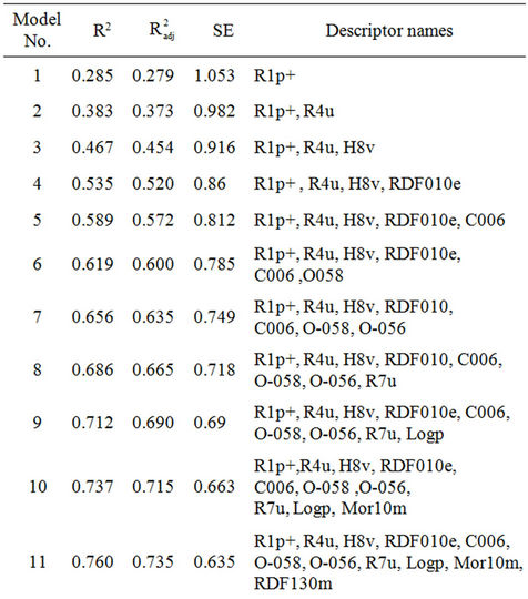
Table 1. Final MLR model summary.
the anti-HIV-1 protease activity (log 1/Ki) relationships with each group of descriptors separately. Log 1/Ki is the dependent variable and the set of descriptors as independent variables. Then, the “optimal” descriptors for each group were selected and gathered in one group to perform new MLR analysis.
2.4. Principal Components Analysis (PCA)
Collinear descriptors add redundancy to the input data matrix and consequently the performances of the models obtained by using these descriptors would be degraded. PCA and more specifically factor analysis, groups together variables that are collinear to form a composite indicator capable of capturing as much of common information of those indicators as possible. Each factor reveals the set of variables with the highest relationship. The idea under this approach is to explain the highest possible variation in the indicators set using the smallest possible number of factors. Consequently, the index no longer depends upon the dimensionality of the data set but it is rather based on the “statistical” dimensions of the data. Application of PCA on a descriptor data matrix results in a loading matrix containing factors or PCs, which are orthogonal and therefore have no correlation with each other.
The PC’s were calculated by singular value decomposition (SVD) method in MATLAB environment (MathWork Inc. Version 7.0.1 (R14)). Due to the quality of data, a previous treatment of the data is essential before applying the multivariate analysis methods. Scaling and centering is one of the pre-processing methods needed before performing the regression methods joint with feature extraction. Projection methods results depend on the normalization of the data. Descriptors with small absolute values have a small contribution to overall variances leading to biased PC’s caused by the presence of other descriptors with higher values. In order to have the focus on the important variables in the model, equal weights are assigned to each descriptor, with appropriate scaling. Furthermore, descriptors were standardized to unit variance and zero mean (autoscaling) to give all variables the same importance. Then, the data matrix containing the entire set of descriptors and activity were simultaneously subjected to PCA.
2.5. Principal Component-Artificial Neural Network (PC-ANN) Analysis
ANNs are computer-based models in which a number of nodes, also called neurons are interconnected by links forming netlike structure “layers”. A variable value is assigned to every neuron.
There are three kinds of neurons: 1) the input neurons which receive their values from independent variables and constitute the input layer, 2) the hidden neurons which collect values from other neurons, giving a result that is passed to a successor neuron, 3) the output neurons which take values from other units and correspond to different dependent variables, forming the output layer. In this sense, network architecture is commonly represented as I-H-O, where I, H, and O are the number of neurons in the input, hidden, and output layers, respectively [5].
The weights are links between units that condition the values assigned to the neurons. The weights are adjusted through a training process in order to minimize network error. For this, a non-linear transfer function relates the input parameters with the outputs. Commonly neural networks are adjusted, or trained, so that a particular input leads to a specific target output.
In PC-ANN analysis, as a preliminary treatment, the input data (i.e., molecular descriptors) were normalized to have zero mean and unity variance, and then were subjected to PCA before being introduced into the neural network. It should be illustrated that for each MLR resulted model, separate ANN models were developed so that the input’s descriptors were the subsets selected by the stepwise MLR methods. In the case of each MLR model, a feed-forward neural network with back-propagation of error algorithm was constructed to model the activity-structure relationships between the descriptors on one hand and inhibitory activity on the other hand. The model development in ANN and the network architecture is fully described by us [13] and others [14]. The data set was divided into training and external test sets. The test set is used to test the trend of the prediction precision of the model trained at some point of the training evolution. The extracted PC’s for each MLR model were classified homogenously, based on the factors space of the descriptors, into training set (80%) and external test set (20%) according to the PCA and the first two PC’s were plotted against each other (see Figure 1). Afterward, the training set was used to optimize the network performance. The regression between the network output and the observed activity was calculated for the two sets individually. The training function “Tanh” was used to train the network. To find models with lower errors, the ANN algorithm was run many times, with different geometry and initial weights each time.
3. Results and Discussion
3.1. MLR Analysis
In continuation to recent QSAR studies [19-22] done using similar methods including nonpeptide HIV-1PR inhibitors [23], we developed an ANN-QSAR model that describes the anti-HIV activity of a series of compounds using large number of different descriptors. MLR were performed on each one of the 17 groups of descriptors individually (individual approach described in Reference [24] by Deeb) where log 1/Ki is the dependent variable. Stepwise method is used to develop multilinear equation by correlating dependent variable (activity) and the best independent variables. The results of the 17 MLR analyses are summarized in Table S2 in the supporting information.
Next, a new or “final” MLR analysis was performed by correlating the dependent variable (activity) and the optimal descriptors selected from the individual 17 MLR models. Table 1 shows the regression models suggested from the “final” MLR analysis. The number of descriptors in these models is varied between 1 and 11. The highest coefficient of determination (R2) obtained, is 0.760 for a regression model with 11 descriptors (model 11). Table 2 shows a key for the different descriptors used in the final MLR model.
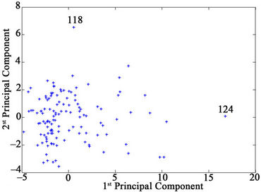
Figure 1. First and second principal components for the factor spaces of the descriptors and anti-HIV-1 protease activity data.
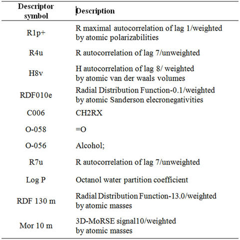
Table 2. Key for the different descriptors used in the final MLR model.
The following equation represents the best MLR model:
Log 1/Ki = 13.443 (±1.450) – 0.376 (±0.108) × C006 – 31.230 (±5.216) ×R1p – 4.665 (±0.539) × R4u –5.871 (±0.905) × H8v + 0.341 (±0.058) × RDF010e + 0.758 (±0.103) × O058 + 0.466 (±0.145) × O056 + 15.911 (±3.928) × R7u + 0.257 (±0.055) × Log P +0.697 (±0.156) × Mor10 m – 0.110(±0.033) × RDF130 m.
According to the above equation, the most important descriptor in this equation is R1p which reflects the polarizability of the compounds; it is inversely proportional to the activity of the compounds. The second important descriptor is R7u which reflects the geometrical matrix of the compound.
Then, leave many out (LMO) cross validation was performed on models 6-11 since these models have coefficients of determination larger than 0.6 [25]. The results of LMO cross validation are summarized in Table S3 in the supporting information. This table shows that the cross-validation coefficient of determination ( ) has positive values starting from model 6 to model 11. Table S3 shows also those models 8-11 have the highest R2 and
  values as well as the lowest root mean square error (RMSE) values. Thus, models 8-11 were chosen for further analysis with ANN.
3.2. PCA
The inputs of the ANN were the subset of the descriptors used in different MLR models (Table 1). First, PCA was performed to classify the molecules into training (80%) and test (20%) sets. Plotting the first and second PC’s, shows that compounds SD146 (molecule 124) and XP- 521 (molecule 118) are outliers (see Figure 1).
This indicates that these 2 molecules behave differently from other molecules with respect to both molecular structure (descriptors) and anti-HIV1 protease activity. Therefore, these molecules are not used in future analysis. According to the pattern of the distribution of the data in factor spaces (Figure 1), the training and test sets molecules were selected homogenously so that molecules in different zones of Figure 1 belong to the two subsets. After removing the outliers and subjecting the data of the remaining 125 molecules to the preliminary treatment mentioned previously, the classified data were used as an input for the ANN.
3.3. ANN
In this study, a three-layered feed-forward ANN model with back propagation learning algorithm [26] was employed. At first, non-linear relationship between the subset of descriptors selected by stepwise selection-based MLR and anti-HIV-1 protease activity was preceded by ANN models with similar structure. The number of hidden layer’s nodes was set to 6 for all models, and the number of nodes in the input layer was the number of descriptors.
The correlation coefficients and cross-validation parameters of ANN analysis for ANN model numbers 8-11 are given in Table S4 in the supporting information. This table shows that the lowest prediction RMSE (RMSEP) is obtained for model 8 while the lowest calibration (training) RMSE (RMSEC) is obtained from model 10. Table S4 in the supporting information shows that model 8 has the highest coefficient of determination for the test set ( = 0.800). However, the calibration and cross validation coefficients of determination for this model are 0.693 and 0.550, respectively.
On the other hand, the highest coefficients of determination for calibration and cross validation are obtained for model 10 ( = 0.796 and
  = 0.734). However, the
  value for this model is 0.772. Hence, these two models were subjected for further analysis by optimizing the number of hidden nodes.
To optimize the performance of the ANN models 8 and 10, these models were trained using different number of hidden nodes starting from 2 to 20. Choosing the best model was based on cross-validation parameters and determination of minimum prediction error [27]. For the evaluation of the predictive ability of a multivariate calibration model, RMSEP is an important statistical parameter to find the best number of hidden nodes. Moreover, because large numbers of hidden nodes often draw attention to the risk of overfitting [28], considering models with low prediction error is avoided if a large number of hidden nodes are used in their network training.
The results of optimizing the number of hidden nodes for models 8 and 10 are summarized in Tables S5 and S6 in the supporting information respectively.
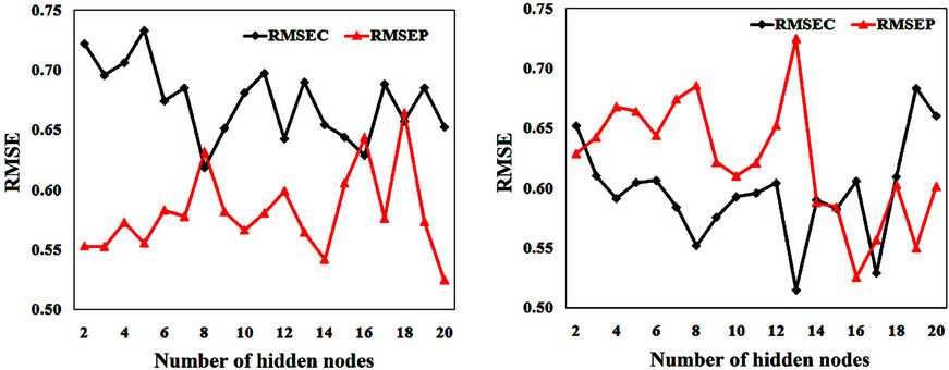
Figure 2(a) shows RMSEC and RMSEP values against the number of hidden nodes for model 8. This figure shows that the lowest RMSEC (0.619) is obtained when using 8 hidden nodes. This value is close to the obtained RMSEP (0.632). Using 8 hidden nodes gives the highest coefficients of determination ( = 0.746 and
  = 0.653). Furthermore, the
  value (0.743) is close to that obtained for the training set.
Figure 2(b) shows RMSEC and RMSEP against the number of hidden nodes for model 10. This figure shows that the lowest RMSEP (0.607) is obtained when using 6 hidden nodes. The RMSEC obtained when using this number of hidden nodes is 0.644. The coefficient of determination obtained for the test set ( = 0.750) is close to that obtained for the training set (
 = 0.756). The
  obtained for this model is 0.675.
 (a) (b)
Figure 2. RMSE of calibration and prediction against hidden nodes number for (a) model 8 and (b) model 10.
Randomization test is performed to investigate the probability of chance correlation for the optimal models (models 8 and 10 with 8 and 6 hidden nodes in the network, respectively). Chance correlation was done using the same configuration parameters and the same activetion functions of all our ANN models. The results of chance correlation for models 8 (using 8 hidden nodes) and 10 (using 6 hidden nodes) are summarized in Tables S7 and S8 in the supporting information, respectively. These tables show that the coefficients of determination obtained by chance are low in general while the RMSE values are high. This indicates that the models obtained from ANN are better than those obtained by chance.
Model 10 has higher coefficients of determination and lower RMSEP than those obtained for model 8. Furthermore, the optimal number of hidden nodes obtained for model 10 (6 hidden nodes) is smaller than that obtained for model 8 (8 hidden nodes). However, the differences between the two models are not large.
As we can see, our models were validated by calculateing different statistical parameters, using external test set and finally performing randomization test.
Figure 3(a) shows plot of the predicted activity against observed ones for the training and test sets compounds of model 8 while Figure 3(b) shows their residuals. Similarly, Figure 3(c) shows plot of the predicted activity against observed ones for the training and test sets compounds of model 10 while Figure 3(d) shows their residuals.
Correlation between calculated and observed log (1/Ki) for the training set of model 8 is given by:
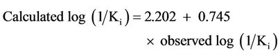 (1)
(1)
and for the test set of this model is given by:
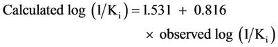 (2)
(2)
while the correlation between calculated and observed log (1/Ki) for the training set of model 10 is given by:
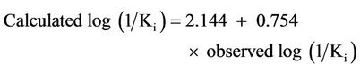 (3)
(3)
and for the test set of this model is given by:
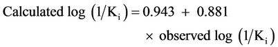 (4)
(4)
To check the presence of outliers in a model, for the training and test sets, the standard deviation of the observed activity data was calculated. The residue which is equal to the difference between the predicted and observed one were calculated also. Finally, if the value of the residue is larger than two times the standard deviation of the observed activity, then this point is considered as an outlier. We found that there was no outlier in our data.
4. Comparison with Other QSAR Studies
Speranta, et al. [18] have performed QSAR study on the same dataset of anti-HIV-1 protease compounds used in this study. They have modeled the HIV-1 protease inhibitor activity (log 1/Ki) from different families using Comparative Molecular Field Analysis (CoMFA) methodology. They found that no simple or multiple regressions gave any statistically significant model. They have obtained  of 0.63 and R2 of 0.70.
Khedkar, et al. [16] used comparative molecular field analysis (CoMFA) and comparative molecular similarity indices analysis (CoMSIA) to build QSAR models for 54 compounds out of 127 compounds used in this study.
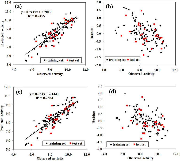
Figure 3. (a) Plot of the predicted anti-HIV-1 protease activities against observed ones and (b) their residuals for model 8; (c) Plot of the anti-HIV-1 protease activities against observed ones and (d) their residuals for model 10.
Two different alignment schemes viz. receptor-based and atom-fit alignment, were used to build the QSAR models. The  values for CoMFA and CoMSIA derived from receptor-based alignment were 0.68 and 0.65, respectively.
Higher calibration and cross validation coefficients of determination were obtained in this study. However, the results obtained by Speranta and Khedkar are for one group of compounds that have the same core structure while in this study, an ANN-QSAR model was built for one heterogeneous group of compounds that contains many families of anti-HIV-1 protease compounds without splitting them into families. The ANN approach used in this study succeeds to explain the non-linear relationships for the data of interest considering the nature of the heterogeneous data set. Although our results seems to be close to Separanta and Khedkar results, our models are more predictive because we used more compounds with different core structures in our data, also we calculated a wider range of descriptors.
5. Conclusions
The performance of the ANN modeling method combined with the individual [24] factor selection approach is applied to predict the anti-HIV inhibitory activity of a set of 127 compounds. The optimal two models have calibration and prediction coefficients of determinations of 0.746 and 0.756. The lowest RMSEP obtained is 0.607. ANN provides improved models for heterogeneous data sets without splitting them into families and gives good regression models with good prediction ability.
Generally, the models obtained from the ANN analysis are better than those obtained by MLR analysis. Both the external and cross-validation methods are used to validate the performances of the resulting models. Employed randomization test indicates that the models obtained from ANN are better than those obtained by chance.
6. Acknowledgements
The authors acknowledge funding support from Al-Quds University.
REFERENCES
- N. E. Kohl, E. A. Emini, W. A. Schleif, L. J. Davis, J. C. Heimbach, R. A. Dixon, E.M. Scolnick, I. S. Sigal, “Active Human Immunodeficiency Virus Protease is Required for Viral Infectivity,” Proceedings of the National Academy of Sciences, Vol. 85, No. 13, 1988, pp. 4686- 4690. doi:10.1073/pnas.85.13.4686
- T. J. McQuade, A. G. Tomasselli, L. Liu, V. Karacostas, B. Moss, T. K. Sawyer, R. L. Heinrikson and W. G. Tarpley, “A Synthetic HIV-1 Protease Inhibitor with Antiviral Activity Arrests HIV-Like Particle Maturation,” Science, Vol. 247, No. 4941, 1990, pp. 454-456. doi:10.1126/science.2405486
- D. R. Davies. “The Structure and Function of the Aspartic Proteinases,” Annual Review of Biophysics and Biophysical Chemistry, Vol. 19, No. 1, 1990, pp. 189-215. doi:10.1146/annurev.bb.19.060190.001201
- A. Wlodawer and J. W. Erickson, “Structure-Based Inhibitors of HIV-1 Protease,” Annual Review of Biochemistry, Vol. 62, No. 1, 1993, pp. 543- 585. doi:10.1146/annurev.bi.62.070193.002551
- M. Fernandez and J. Caballero, “Modeling of Activity of Cyclic Urea HIV-1 Protease Inhibitors Using RegulariZed-Artificial Neural Networks,” Bioorganic & Medicinal Chemistry, Vol. 14, No. 1, 2006, pp. 280-294. doi:10.1016/j.bmc.2005.08.022
- N. A. Roberts, J. A. Martin, D. Kinchington, A. V. Broadhurst, J. C. Craig, I. B. Duncan, S. A. Galpin, B. K. Handa, J. Kay, A. Kroehn, R. W. Lambert, J. H. Merrett, J. S. Mills, K. E. B. Parkes, S. Redshaw, A. J. Ritchie, D. L. Taylor, G. J. Thomas and P. J. Machin, “Rational Design of Peptide-Based HIV Proteinase Inhibitors,” Science, Vol. 248, No. 4953, 1990, pp. 358-361. doi:10.1126/science.2183354
- O. Aruksakunwong, S. Promsri, K. Wittayanaraku, P. Nimmanpipug, V. S. Lee, A. Wijitkosoom, P. Sompornpisut and S. Hannongbua, “Current Development on HIV-1 Protease Inhibitors,” Current Computer-Aided Drug Design, Vol. 3, No. 3, 2007, pp. 201-213. doi:10.2174/157340907781695431
- D. C. Montgomery and E. A. Peck, “Introduction to Linear Regression Analysis,” Wiley, New York, 1982.
- G. Schneider and P. Wrede, “Artificial Neural Networks for Computer-Based Molecular Design,” Progress in Biophysics and Molecular Biology, Vol. 70, No. 3, 1998, pp. 175-222. doi:10.1016/S0079-6107(98)00026-1
- P. J. Gemperline, J. R. Long and G. Gregoriou, “Nonlinear Multivariate Calibration Using Principal Components Regression and Artificial Neural Networks,” Analytical Chemistry, Vol. 63, No. 20, 1991, pp. 2313-2323. doi:10.1021/ac00020a022
- R. Vendrame, R. S. Braga, Y. Takahata and D. S. Galvao, “Structure-Activity Relationship Studies of Carcinogenic Activity of Polycyclic Aromatic Hydrocarbons Using Calculated Molecular Descriptors with Principal Component Analysis and Neural Network Methods,” Journal of Chemical Information and Modeling, Vol. 39, No. 6, 1999, pp. 1094-1104. doi:10.1021/ci990326v
- B. Hemmateenejad, M. Akhond, R. Miri and M. Shamsipur, “Genetic Algorithm Applied to the Selection of Factors in Principle Component-Artificial Neural Networks: Application to QSAR Study of Calcium Channel Antagonist Activity of 1, 4-Dihydropyridines (Nifedipine Analogous),” Journal of Chemical Information and Modeling, Vol. 43, No. 4, 2003, pp. 1328-1334. doi:10.1021/ci025661p
- O. Deeb and B. Hemmateenejad, “ANN-QSAR Model of Drug-Binding to Human Serum Albumin,” Chemical Biology & Drug Design, Vol. 70, No. 1, 2007, pp. 19-29. doi:10.1111/j.1747-0285.2007.00528.x
- B. Hemmateenejad, M. A. Safarpour, R. Miri and N. Nesari, “Toward an Optimal Procedure for PC-ANN Model Building: Prediction of the Carcinogenic Activity of a Large Set of Drugs,” Journal of Chemical Information and Modeling, Vol. 45, No. 1, 2005, pp. 190-199. doi:10.1021/ci049766z
- G. Ramírez-Galicia, R. Garduño-Juárez, O. Deeb and B. Hemmateenejad, “PCR-ANN and RTO Approach to L- opioid Receptor-Binding Affinity. Pooling Data from DifFerent Sources,” Chemical Biology & Drug Design, Vol. 71, No. 3, 2008, pp. 260-270. doi:10.1111/j.1747-0285.2008.00626.x
- V. M. Khedkar P. K., Ambre, J. Verma, M. S. Shaikh, R. R. S. Pissurlenkar and E. C. Coutinho, “Molecular Docking and 3D-QSAR Studies of HIV-1 Protease Inhibitors,” Journal of Molecular Modeling, Vol. 16, No. 7, 2010, pp. 1251-1268. doi:10.1007/s00894-009-0636-5
- O. Deeb and M. Goodarzi, “Exploring QSARs for Inhibitory Activity of Non-Peptide HIV-1 Protease Inhibitors by GA-PLS and GA-SVM,” Chemical Biology & Drug Design, Vol. 75, No. 5, 2010, pp. 506-514. doi:10.1111/j.1747-0285.2010.00953.x
- A. Speranta, C. Bologa and M. L. Flonta, “Quantitative Structure-Activity Relationship by CoMFA for Cyclic Urea and Nonpeptide-Cyclic Cyanoguanidine Derivatives on Wild Type and Mutant HIV-1 Protease,” Journal of Molecular Modeling, Vol. 11, No. 2, 2005, pp. 105-115. doi:10.1007/s00894-004-0226-5
- O. Deeb and M. Drabh, “Exploring QSARs of Some Analgesic Compounds by PC-ANN,” Chemical Biology & Drug Design, Vol. 76, No. 3, 2010, pp. 255-262. doi:10.1111/j.1747-0285.2010.01004.x
- P. V. Khadikar, O. Deeb, A. Jaber, J. Singh, V. K. Agrawal, S. Singh and M. Lakhwani, “Development of Quantitative Structure-Activity Relationship for a Set of Carbonic Anhydrase Inhibitors: Use of Quantum and Chemical Descriptors,” Letters in Drug Design & Discovery, Vol. 3, No. 9, 2006, pp. 622-635. doi:10.2174/157018006778341138
- O. Deeb, B. Hemmateenejad, A. Jaber, R. GardunoJuarez and R. Miri, “Effect of the Electronic and Physicochemical Parameters on the Carcinogenesis Activity of Some Sulfa Drugs Using QSAR Analysis Based on Genetic-MLR and Genetic PLS,” Chemosphere, Vol. 67, No. 11, 2007, pp. 2122-2130. doi:10.1016/j.chemosphere.2006.12.098
- O. Deeb, K. M. Youssef and B. Hemmateenejad, “QSAR of Novel Hydroxyphenylureas as Antioxidant Agents,” QSAR and Combinatorial Sciences, Vol. 27, No. 4, 2008, pp. 417-424. doi:10.1002/qsar.200730023
- O. Deeb and M. Goodarzi, “Exploring QSARs for Inhibitory Activity of Nonpeptide HIV-1 Protease Inhibitors by GA-PLS and GA-SVM,” Chemical Biology and Drug Design, Vol. 75, No. 5, 2010, pp. 506-514. doi:10.1111/j.1747-0285.2010.00953.x
- O. Deeb, “Correlation Ranking and Stepwise Regression Procedures in PC-ANN Modeling and Application to Predict the Toxic Activity and HSA Binding Affinity,” Chemometrics and Intelegent Laboratory Systems, Vol. 104, No. 2, 2010, pp. 181-194. doi:10.1016/j.chemolab.2010.08.007
- A. Golbraikh and A. Tropsha, “Beware of q2!” Journal of Molecular Graphics and Modelling, Vol. 20, No. 4, 2002, pp. 269-276. doi:10.1016/S1093-3263(01)00123-1
- D. E. Rumelhart, G. E. Hinton and R. J. Williams, “Learning Representations by Back-Propagating Errors,” Nature, Vol. 323, 1986, pp. 33-536. doi:10.1038/323533a0
- H. Martens and T. Naes, “Multivariate Calibration,” John Wiley, Chichester, 1989.
- E. P. P. A. Derks and L. M. C. Buydens, “Aspects of Network Training and Validation on Noisy Data: Part 1. Training Aspects,” Chemometrics and Intelligent Laboratory Systems, Vol. 41, No. 2, 1998, pp. 171-184. doi:10.1016/S0169-7439(98)00053-7
Supporting Information
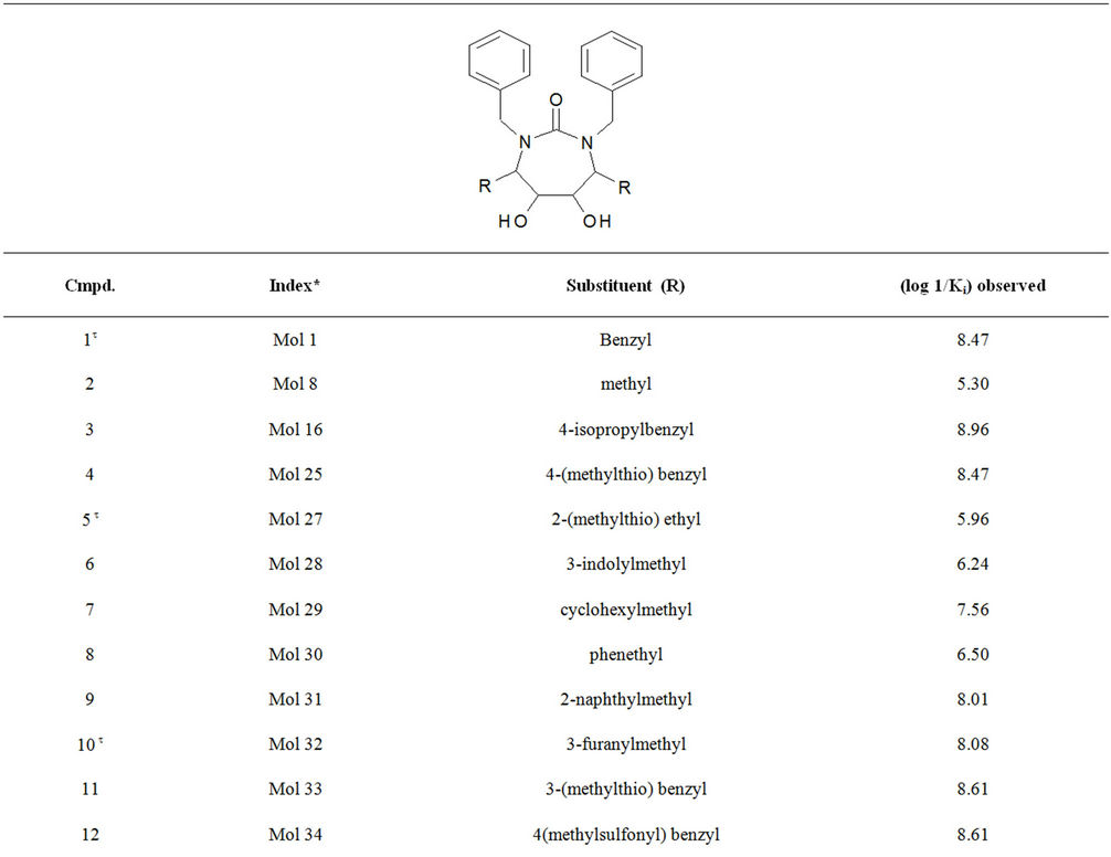
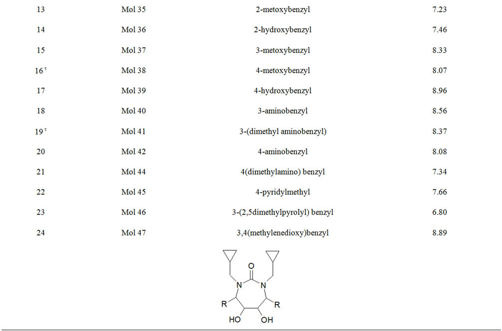
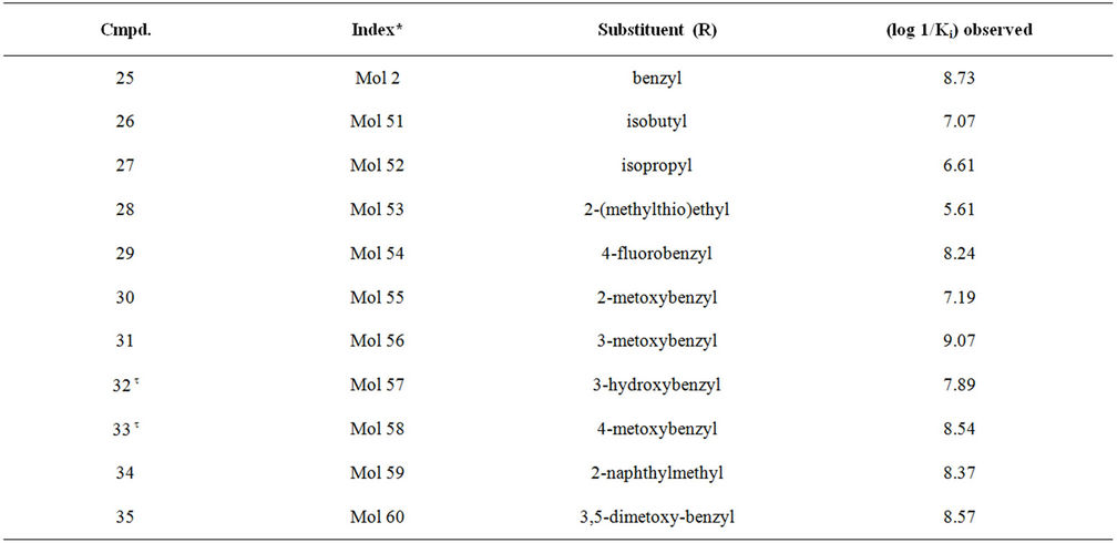
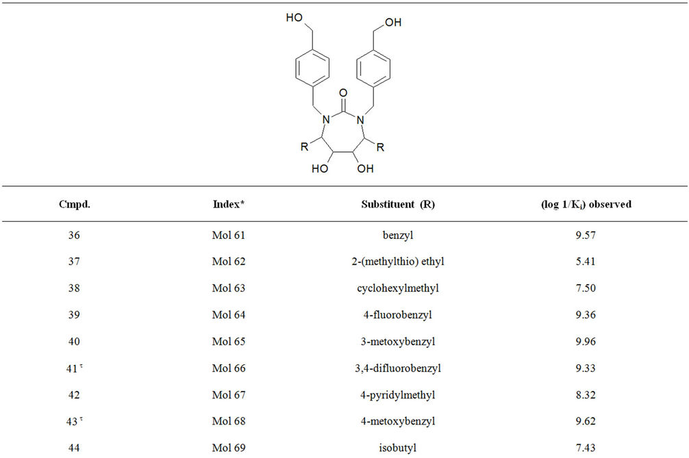
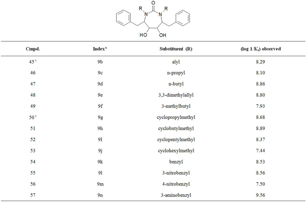
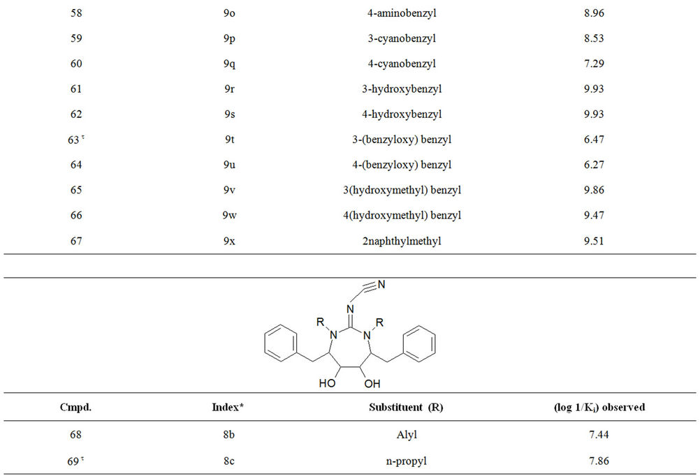
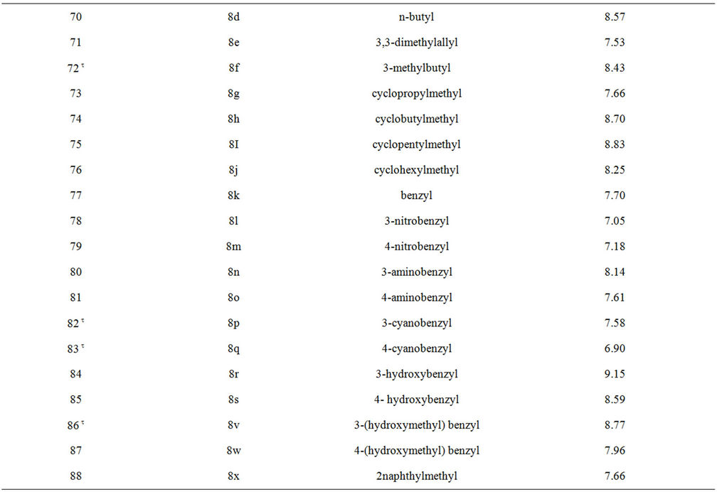
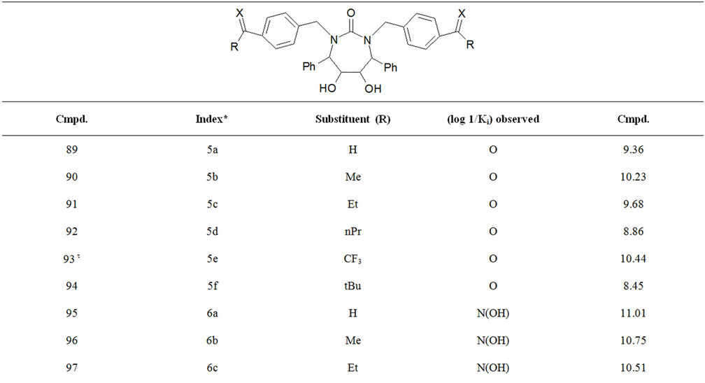
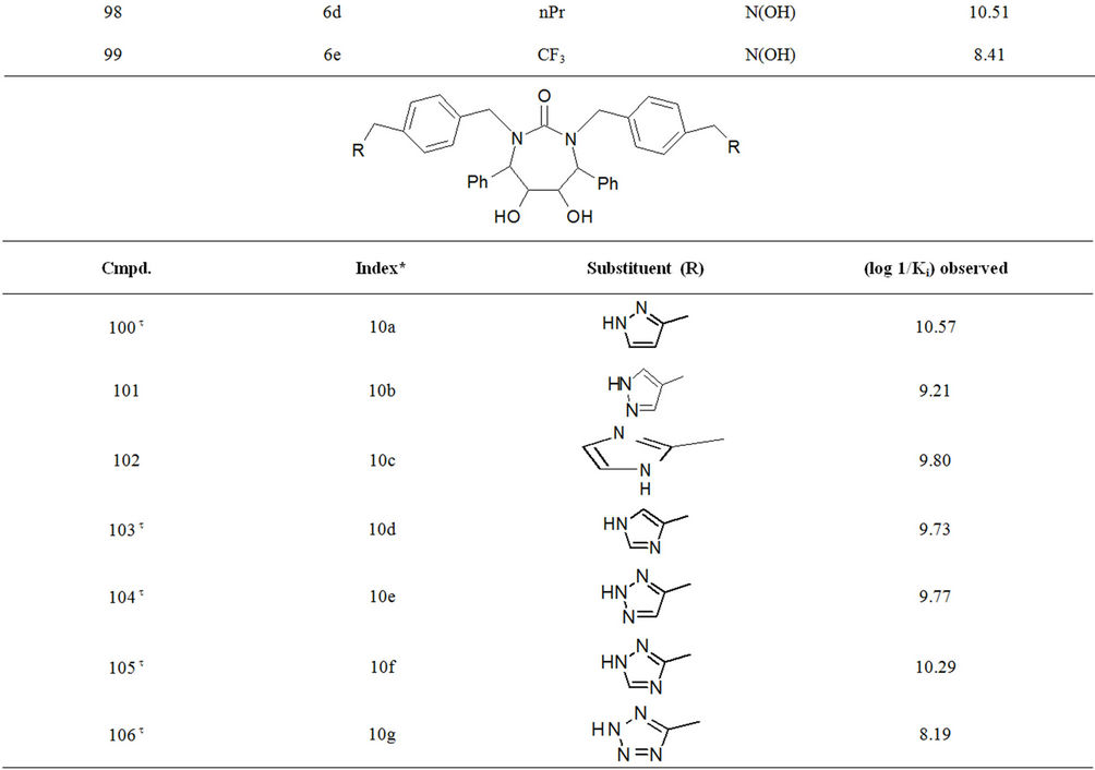
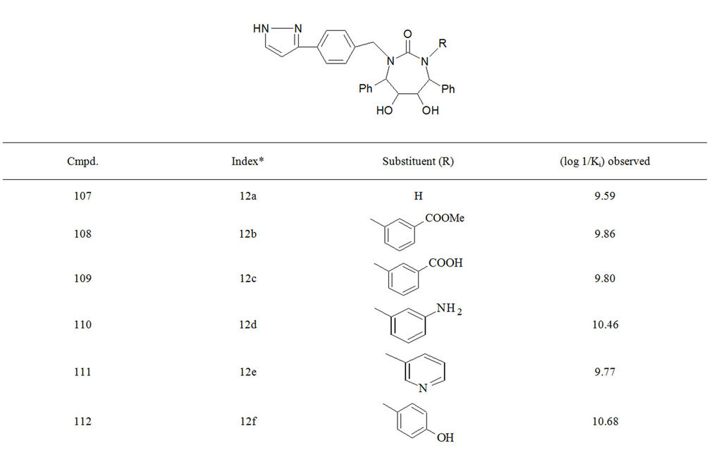
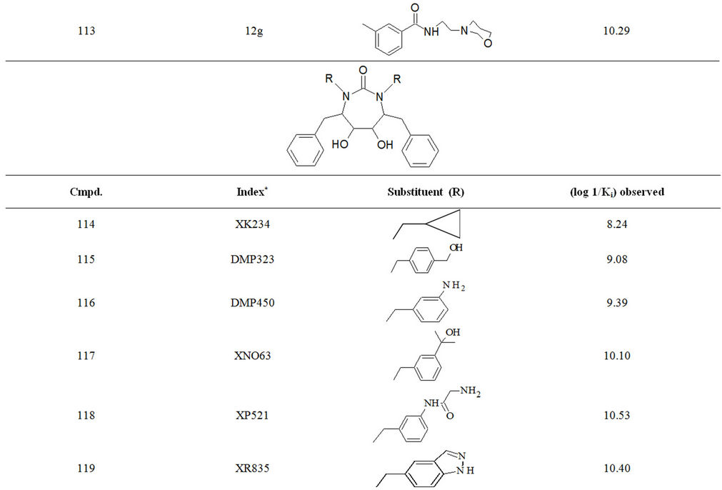
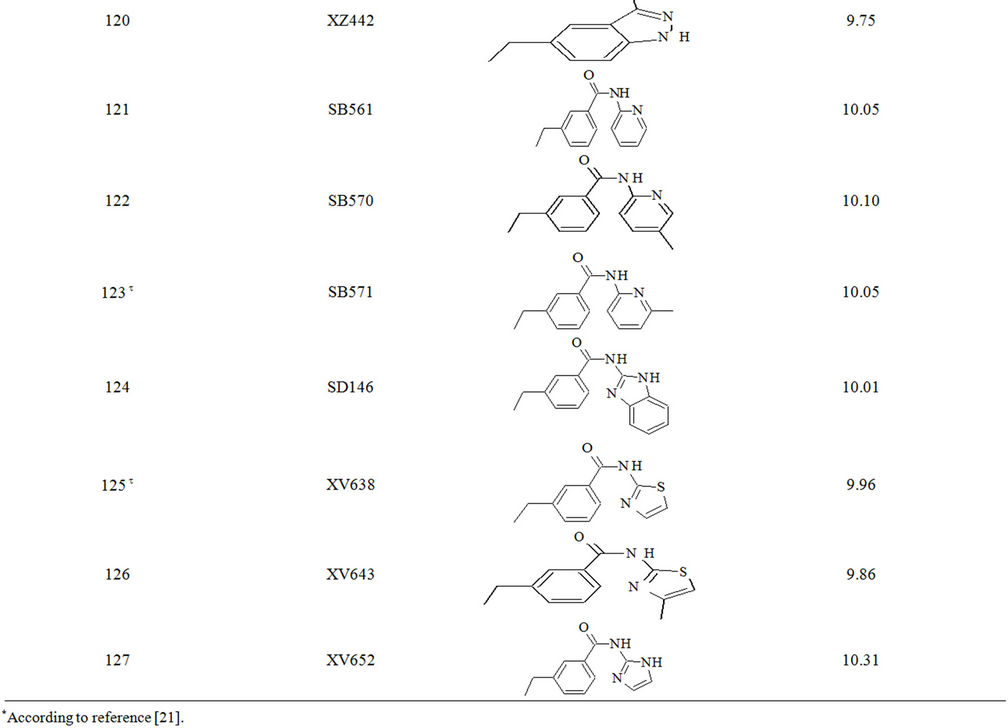
Table S1. Molecular structures and observed activities of the 127 HIV-1 PR cyclic urea and non peptide cyanoguanidine derivative inhibitors expressed as log 1/Ki (R) and (X) in all structures represent the substituent.
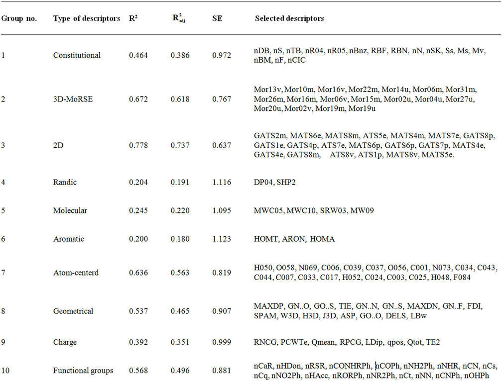
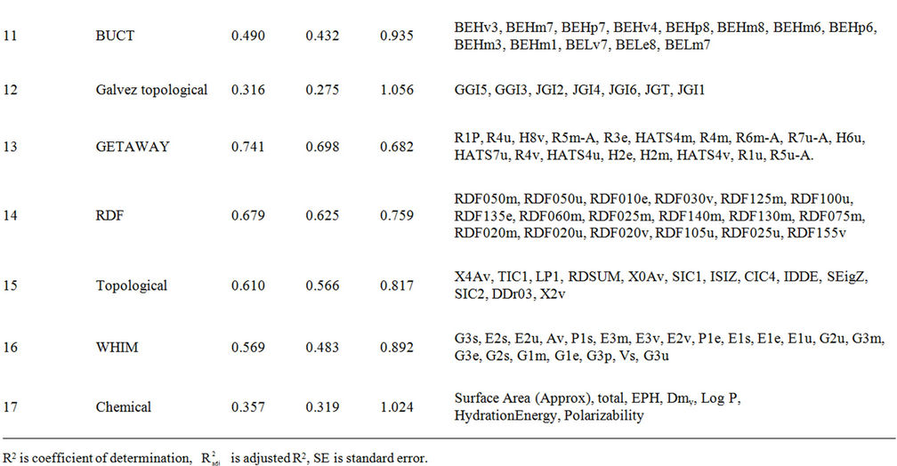
Table S2. Regression models suggested from the 17 MLR analysis; their coefficients of determination and standard error (SE).
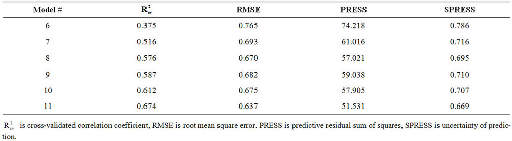
Table S3. LMO cross validation parameters for the final MLR models 6-11.
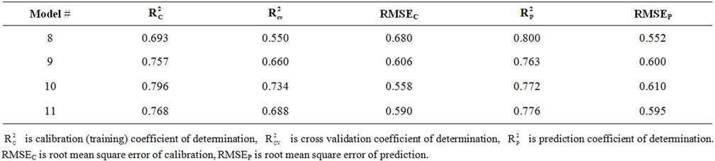
Table S4. Coefficients of determination and cross validation results for ANN models 8-11.
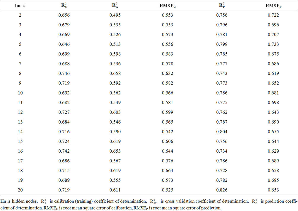
Table S5. Coefficient of determination and cross validation parameters for optimizing number of hidden nodes for model 8.
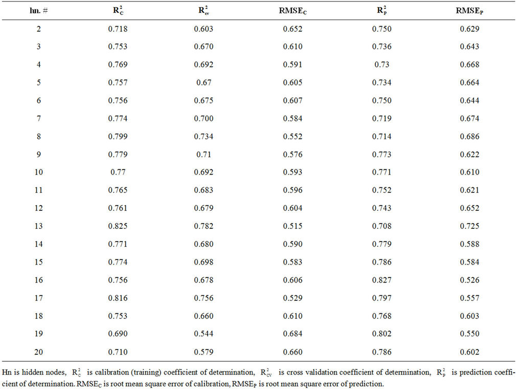
Table S6. Coefficient of determination and cross validation parameters for optimizing number of hidden nodes for model 10.
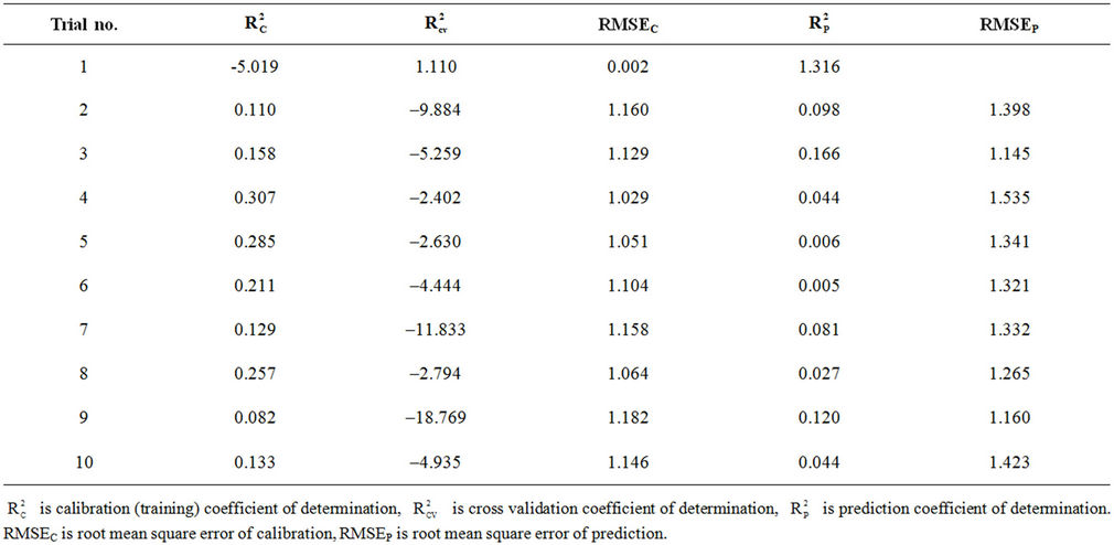
Table S7. Coefficients of determination and cross validation parameters for chance correlation results for model 8 with 8 hidden nodes.
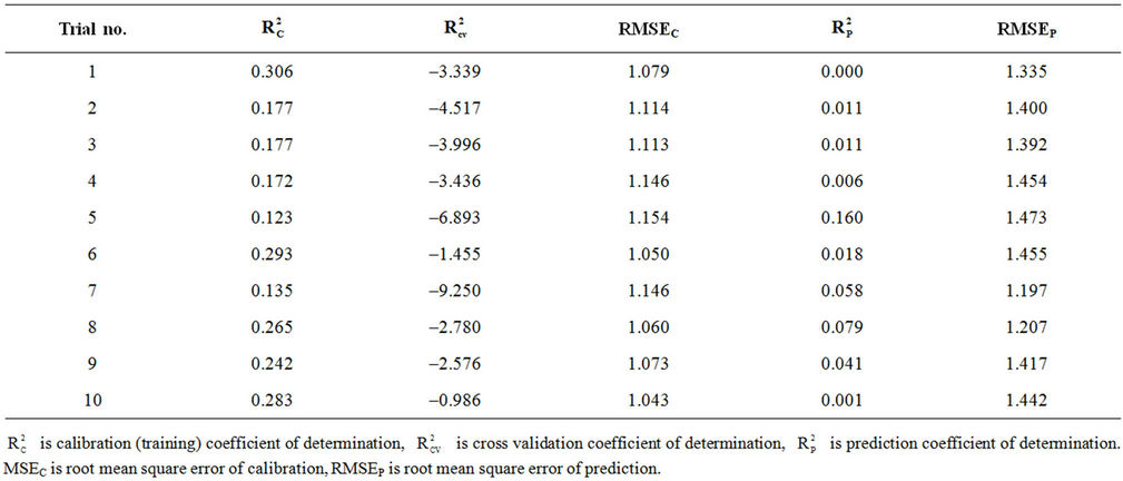
Table S8. Coefficients of determination and cross validation parameters for chance correlation results for model 10 with 6 hidden nodes.
NOTES
*Corresponding author.