Journal of Signal and Information Processing
Vol. 3 No. 2 (2012) , Article ID: 19568 , 10 pages DOI:10.4236/jsip.2012.32027
A New Useful Biometrics Tool Based on 3D Brain Human Geometrical Characterizations
![]()
1LTSIRS Laboratory, National Engineering School of Tunis, Belvedere, Tunisia; 2Université Paris-Est, Créteil, France.
Email: {aloui_meteo, naceurs}@yahoo.fr, *naitali@u-pec.fr
Received August 5th, 2011; revised September 22nd, 2011; accepted January 17th, 2012
Keywords: Brain; MRI; Cortex; Cortical Folding; Level-Sets; Biometrics; Projection; Curvature; Brain
ABSTRACT
Previous clinical research studies consider the existence of differences among normal individual cerebral cortex and show that some features such as cerebral sulci are unique for each individual so that human brains are anatomically different and unique to each individual. In this work, we highlight the idea which consists in using medical data, such as brain MRI images for the purpose of individual identification or verification. In other words, we raise the following question: can one identify individuals using their brain geometry characteristics? Our aim is to validate the feasibility of this new biometrics tool based on human brain characterization. The proposed approach differs from existent biometrics modalities (e.g. fingerprint, hand, etc.) in the sense that brain features cannot be modified by individuals as it is the case when using fake fingerprints, or fake hands. In this work, we consider volumetric Magnetic Resonance Images (MRI) from which brain shapes are extracted using a 3D level-sets segmentation approach. Afterwards, geometrical descriptors are extracted from the 3D brain volume and from a projected version which provide specific features such as the isoperimetric ratio, the cortical surface curvature and the Gyrification index. Evaluations performed on a set of MRI images obtained from (MeDEISA) database show that it is possible to distinguish between individuals using their brain characteristics. Preliminary results are particularly encouraging.
1. Introduction
From a macroscopic point of view, the brain requires various phases during its evolution up to the maturation (from a totally smooth brain to a highly wrinkled brain [1, 2]). According to the appearance date of the folding, their shape, and their variability; three types of cortical folding can be distinguished, namely: 1) the primary folding, characterized by a weak inter-individual variability, visible from the 16th week of gestation [3], 2) the secondary type of folding, characterized by an intermediate level variability which appears at about the 32nd week of gestation establishing the Gyrification degree of the cerebral cortex, and 3) the tertiary folding types, characterized by a high inter-individual variability, developed at about the 36th week of gestation. Numerous anatomical studies of the human brain consider a partitioning into different areas which are often delineated by folds, showing a significant inter-individual variability of the geometric shape. In addition, studies have shown that the two hemispheres of a same individual are not necessarily symmetrical and that inter-hemispheric variability show that the geometric shape of the cerebral cortex is unique for each individual [4-6]. In such a context, we believe that an objective quantification of human brains could contribute considerably in biomedical and biometrics research areas so that one can provide a new useful tool to identify individuals through their cerebral signatures.
The proposed approach differs from some well known common modalities such as fingerprint recognition, iris, face, etc., in the sense that the proposed modality is not subject to external modifications (e.g. minor injuries) except in pathological cases, not considered in this work. Moreover, the proposed technique doesn’t allow any type of fakes as it is the case when dealing with classical techniques. “No one can change the feature of his own brain”. This approach can also be employed for the purpose of cadaver identification, obviously under some specific body conservation conditions and before using any DNA identification.
Except direct post-mortem characterizations of the cerebral cortex, the Magnetic Resonance Imaging (MRI) is potentially a very attractive approach to study the anatomy of the cerebral cortex. This biomedical imaging technique allows a good visualization of different anatomical structures such as cortical sulci and it becomes more flexible to use thanks to the recent development of high-performance computers allowing a fast implementation of three-dimensional processing algorithms. Actually, from the literature, several research studies have been dedicated especially to clinical purposes such as: the asymmetry of the brain; the neurological morphometry (e.g. autism); the schizophrenia, etc.
As it has been evoked previously, our objective is not clinical since we aim to quantify differences between the cerebral cortex of normal individuals for the purpose to study the possibility of identifying individuals through their brain signature. Consequently, we define in this work, through two approaches, new geometrical descriptors of adult and healthy human brains. In the first approach, the brain is represented through 3D triangular meshes, whereas in the second approach, the brain volume is projected so that one can obtain three views, namely: axial, coronal and sagittal views. From each view, geometrical parameters are extracted. Therefore, three feature vectors are obtained (x, y and z) containing respectively L, M and N parameters characterizing the brain. To evaluate our method, MRI volumetric images are provided from the database “Medical Database for the Evaluation of Image and Signal Processing Algorithms”, MeDEISA [7].
This paper is organized as follows: in Section 2, we present the kernel of our method which consists in: 1) segmenting 3D MRI images using a level-set based method in order to extract the brain geometry, 2) estimating brain features “geometrical descriptors” from a 3D representation, 3) estimating brain features from a projected representation providing, coronal (front), axial (top) and sagittal (lateral) views. In Section 3, objective results are presented and commented. Finally, a discussion and a conclusion related to this work are given in Section 4.
2. Proposed Method
Segmenting manually volumetric images is a complex process which requires lot of time and much concentration to achieve a good quality extraction of regions of interest. Actually, structures of interest show weak contrast and high noise at boundaries since they are made of anatomical tissues mixtures (i.e. CerebroSpinal Fluid (CSF), Grey Matter (GM) and White Matter (WM)). For this reason, it is generally interesting to deal with automatic segmentation algorithms. For this purpose, a range of methods including edge based, region based, and knowledge based have been proposed for semi-automatic or automatic detection of various anatomical brain structures. Recently, several attempts have been made to apply deformable models [8-10] to brain image analysis. Indeed, deformable models refer to a large class of computer vision methods and have proved to be successful segmentation techniques for a wide range of applications. Moreover, they constitute an appropriate framework for merging heterogeneous information and they provide a consistent geometrical representation suitable for a surface based analysis.
In some particular Level-sets [11], geometric deformable models provide an elegant solution for medical image processing, especially for normal brain segmentation [12-15]. In this paper, to extract brain shape from volumetric MRI images we will use a region-competition level-set method as described in [16,17]. This algorithm overcomes classical level-set problems by modulating the propagation term with a signed local statistical force, leading to a stable solution.
2.1. Region-Competition Based Level-Set
We propose a method which operates on 3D MRI scans of the human brain to segment the brain tissue. First, the data volume is pre-processed with an anisotropic diffusion filtering method [18] to reduce the noise and preserve edges. Then no-brain tissues are removed from the data volume by a simple thresholding. Afterwards, a 3D binary morphological erosion and dilation process [19] are applied to get an initial brain surface and finally we refine brain region extraction by using region-based information into the level set framework. These computational steps are illustrated in Figure 1.
The aim of the third step is to extract “exactly” the cerebral cortex surface representing the interface between MG and CSF. For this reason, we propose to use a deformable model algorithm based on the level set technique. We propose also to drive our model by region information instead boundary information, because it is more robust. The process requires an initialization step and the definition of image forces to guide the propagation direction and speed up the level-set. Theoretically, the level-set snake is defined as the zero level set of an implicit function  defined on the entire volume. This function will change over the time according to the speed term F. The evolution of
  is defined as in [11] via a partial differential equation:
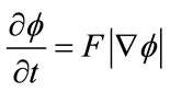 (1)
(1)
The classical speed term is defined as in [20,21]:
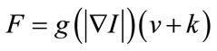 (2)
(2)
where  is the stop function that limits the propagation force to zero as the edge strength increases. The curvature
  and the constant force
  propagate curve to the region of interest surface.
In this work, we use a simplified version of the levelset formulation [17]. The model shrinks when the boundary encloses parts of the background, and grows when
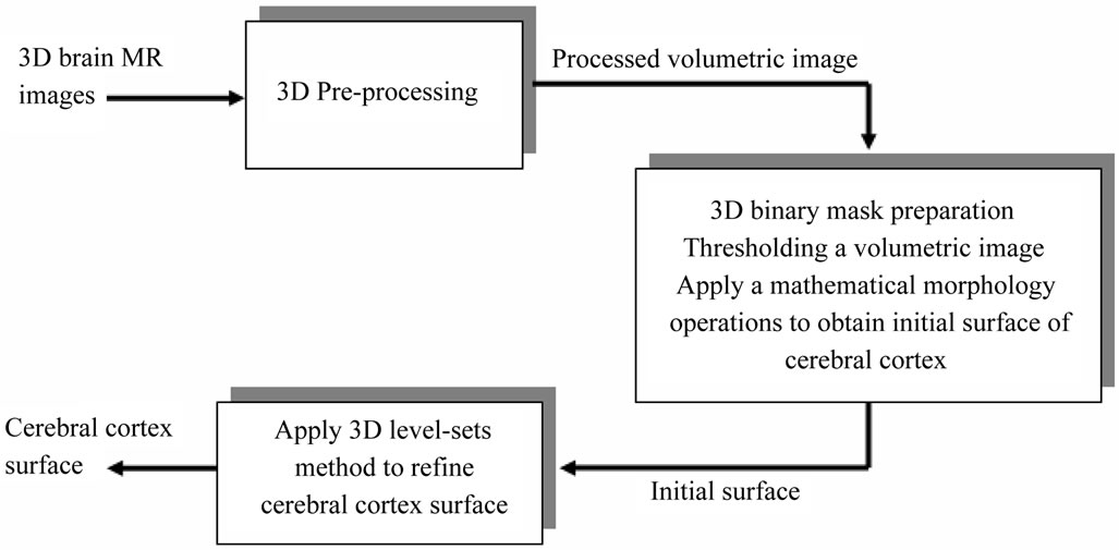
Figure 1. Proposed method for brain cortical surface segmentation.
the boundary is inside the brain region. Here, the speed function usually consists in a combination of two terms: curvature term for smoothness and data term for evolution. The snake evolves using the following equation:
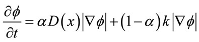 (3)
(3)
where D is a data term that forces the model to expand or contract toward desirable features in the input data. By making D positive in desired regions or negative in undesired regions. The term k is the means curvature of the surface, which forces the surface to have less area (and remain smooth), and  is a free parameter that controls the degree of smoothness.
The speed function depends on the grayscale value input data  at the point
 :
:
 (4)
(4)
where  controls the brightness of the region to be segmented and
  controls the range of grayscale values around
  that could be considered inside the object. A model situated on voxels with grayscale values in the interval
  will expand to enclose that voxel, whereas a model situated on grayscale values outside that interval will contract to exclude that voxel.
As represented in Figure 2,  describes the central intensity value of the region to be segmented, and
  describes the intensity deviation around
  that is a part of the desired segmentation. Therefore if a pixel or voxel has an intensity value within the
  range, the model will expand; otherwise it will contract.
Consequently, the three user parameters that need to be specified for the segmentation are ,
,  and
and . An initial mask to be transformed to a signed distance [22] for the level-set function is also required (Figure 3). The level set iteration can be terminated once
  has converged, or after a certain number of iterations.
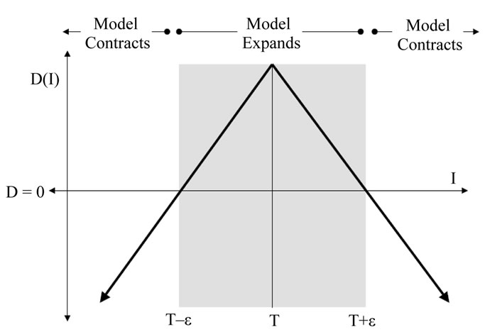
Figure 2. The speed term from [17].

Figure 3. Cerebral cortex surface obtained after 3D segmentation of volumetric brain MR Images [6]. (a) Initial cerebral cortex surface; (b) Show 2D projection into 2D brain slice of initial surface; (c) Cerebral cortex surface obtained using 3D level-sets method; (d) 2D projection of brain refined surface into 2D brain slice.
2.2. 3D Geometrical Cerebral Cortex Characterization
When dealing with the characterization aspect of 3D object, we generally refer to extracting distinctiveness descriptors or measures of shape variability. For example, if we ask for the difference between a foot ball and a rugby ball, one can answer that the first one is more round than the second one. By analogy, we provide in this section a measure of this difference applied on the human brain shape. The application of mathematics of differential geometry to their shape analysis has been shown to be useful in [23,24].
The proposed method is described as follows: we define various invariants geometrical descriptors for the cerebral cortex surfaces [25-30]. For this purpose, we have achieved seven measures, validated using a collection of magnetic resonance scans of eight normal adult subjects. These measures quantify the amount of the surface area in a given volume, namely, the convexity of the surface, the intrinsic and extrinsic curvatures, the minimal, and the maximal and mean distances separating the cerebral cortex surface regarding the surface centre of gravity.
1) Isoperimetric Ratio (IPR): the isoperimetric ratio (IPR) is defined by 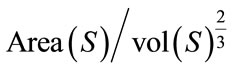 where Area(S) is the surface area, and the vol(S) is the brain volume. This descriptor measure the failure of the brain surface to be a sphere. We also define the convex isoperimetric ratio (IPRconv), which can be calculated by
 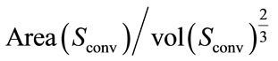 representing the relationship between the area and the volume delimited by convex hull surface of the cerebral cortex.
2) Convexity Ratio (CR): the CR takes its minimum for convex bodies. In other words, this descriptor measures the failure of the brain shape to be convex. We defined two measures, namely, the surface area convexity ratio (CRS), which is defined by  and the volume convexity ratio (CRV) defined by
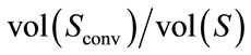 .
.
3) Gyrification Index (IG): the IG descriptor is a 2D convexity ratio (CR) which is considered as a slice-byslice version of the SCR. It is the ratio of inner to outer cortical contours, see [28,29].
4) Gauss and Mean Curvature L2 Norm: measures, given above which are based on the surface area or the volume enclosed do not require differentiable patches. In such a context we have defined two different measures based on differentials features of discrete surface like the principal curvatures kmin and kmax or the Gauss and mean curvatures, K and H, [24,26]. These pairs of measures are related by the following expression: 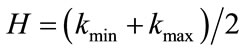 and
and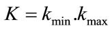 . Gauss curvature L2 Norm is L2 Norm which we normalize by the square root of the surface area divided by
 , which we call
  . The Mean curvature L2 Norm (MLN) is
 . The GLN descriptor measure of how much of the surface has constant Gauss curvature and the MLN descriptor as a measure of bending of the cortex surface.
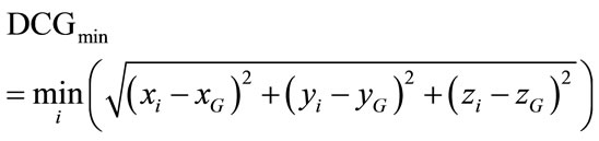
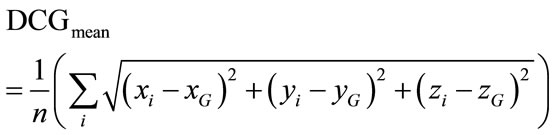
5) A Point Cloud Descriptors: cerebral cortex surface is a set of vertices in a three-dimensional coordinate system. These vertices are defined by X, Y and Z coordinates. The descriptors we used are derived from the characterization of 3D point cloud representing the brain surface to measure the variability of the human brain shape. We defined here three descriptors from the point cloud, namely, minimal, maximal and mean distances separating the cerebral cortex surface regarding the surface centre of gravity. They are expressed respectively by:
 (5)
(5)
 (6)
(6)
 (7)
(7)
where n, is the number of vertexes in brain meshes surface and  is the centre of gravity of cerebral cortex meshes surface defined by:
 (8)
(8)
2.3. 2D Characterization of a Projected Cerebral Cortex
Geometric descriptors of human brain shape, given above are based on the characterization of 3D cortical surface. The idea presented in this sub-section consists in exploring a new approach which characterizes the brain geometry using a three parameters descriptor. These three parameters are indeed obtained by projecting the brain according to three directions (Figure 4) producing hence the coronal, axial and sagittal views. From each view, geometrical parameters are extracted. Therefore, three feature vectors are obtained (x, y and z) containing respectively L, M and N parameters characterizing the brain shape. For each view (2D surface) we defined some measures, namely, the maximal distance separating brain
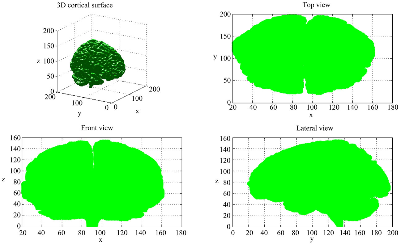
Figure 4. Cerebral cortex surface 2D projection on coronal, axial and sagittal views.
projected view regarding the centre of gravity, called DMAX; the minimal distance called DMIN, the mean distance called DMEAN and the surface-perimeter ratio called SP.
These descriptors will be evaluated in the next section.
3. Results
To evaluate the proposed approach, MRI volumetric images have been used. They can be downloaded from the well known MeDEISA database “Medical Database for the Evaluation of Image and Signal Processing Algorithms” [7].
Results corresponding to the 3D characterisation and the 2D characterisation of the projected cerebral cortex are considered below, respectively in sub-Sections 3.1 and 3.2.
3.1. 3D Geometrical Cerebral Cortex Characterization
Based on the features considered in Section 2.1, Table 1 shows the mean value, minimal and maximal value and standard deviation for each descriptor that describes 3D geometrical shape of eight brains. These statistical values indicate the variation range of each descriptor. Specifically, the most significant descriptors having the ability to describe inter-individual shape variability of cerebral cortex are those characterized by a wide range of variation and from which we can distinguish and differentiate brains. One can notice that the MLN (s = 32.06) and
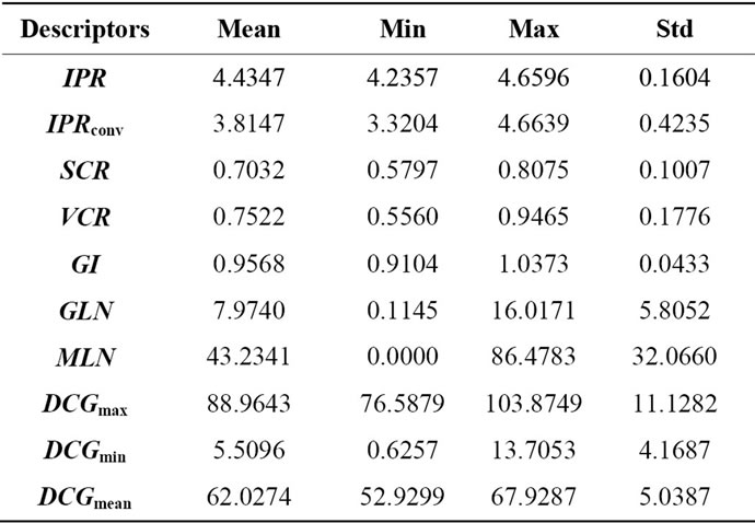
Table 1. 3D geometrical cerebral cortex characterization.
DCGmax (s = 11.19) are the most significant descriptor to characterize geometrical shape of the cerebral cortex. The two selected descriptors do not eliminate the ability of other descriptors to describe 3D geometrical brain shape. In fact, to identify a person through the brain signature requires multiple parameters for more reliable identification procedure, so all descriptors in Table 1 can be used in a hierarchical identification according to a descriptor weight whose purpose is to refine signatures brain matching and recognition.
3.2. 2D Characterization of the Projected Cerebral Cortex
These geometrical descriptors, as described in Section 2.2, are evaluated on the same set of MRI volumetric images used in the previous sub-section. Consequently, results from Tables 2, 3 and 4 show respectively the mean value, minimal and maximal value and standard deviation for each descriptor that describes coronal (front), axial (top) and sagittal (lateral) views of brains surface. The measures corresponding to each descriptor and to each brain views characterized by a wide range of variation and from which we can distinguish and differentiate brains shape.
Unlike the direct volume characterization, this approach seems to be more flexible for brain print recognition and matching to distinguish between individuals. This new approach of brain views characterization provides more degree of freedom to identify individuals using their brain geometry characteristics. For more reliable identification procedure we can use a vectorial analysis. In other words, for individual identification based on geometric brain shapes, it is more appropriate to use a set of descriptors (L, M and N parameters) instead a scalar analysis on each projection brain view.
Geometrical descriptors characterizing each brain views can be either correlated or not. In fact in this proposed approach one can expect that better results can be obtained by combining descriptors for each brain views. For instance, one can include inter-views correlation. In other words, we can use new descriptors of brain shape from inter views correlation such as:
o 
o 
o  .
.
To identify a person through the brain signature it is more appropriate to use multiple parameters for more reliable identification procedure. In fact the idea is to assign to each individual a vector of geometric descriptors for each view of his brain and a vector of descriptors from the correlation between sagittal, axial and coronal view. Consequently, higher is the dimension of the brain vectors descriptors better is the capacity to distinguish between individuals.
4. Discussion and Conclusions
The objective of this work consists in studying the feasibility of a new biometrics technique, completely different compared to classical techniques (e.g. fingerprint, iris, face recognition, etc.). The proposed modality consists in using human brain geometry for the purpose of identifying individuals. The main advantage of this modality is that the acquired data cannot be subject to any voluntary modification (i.e. no one can change the geometry of his own brain). As reported in the abstract of this paper, this technique seems to be complex to be used in daily identification routines, but we believe that regarding technological progresses, such processes could be easier to
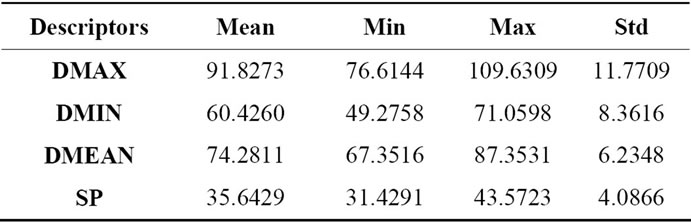
Table 2. Geometrical characterization of 2D cerebral cortex projection axial view.

Table 3. Geometrical characterization of 2D cerebral cortex projection coronal view.
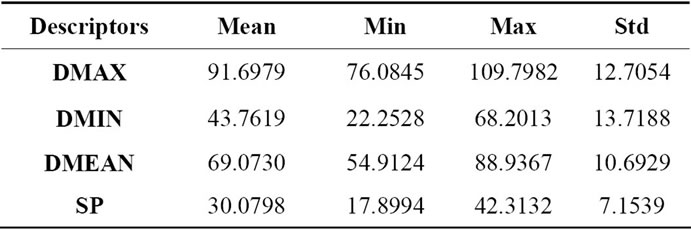
Table 4. Geometrical characterization of 2D cerebral cortex projection sagittal view.
employ in the future.
Using seven volumetric MRI images obtained from MeDEISA database, a first approach based on a 3D brain modelling has been employed. Each volume is segmented using a 3D level set algorithm, then ten various measures have been evaluated. Results show that the MLN and DCGmax are the most significant descriptor that can be used to characterize geometrical shape of the cerebral cortex. Whereas, the others descriptors such as GLN, DCGmin and DCGmean can be used to refine the identification.
The second proposed approach consists in projecting a given volume according to three directions, namely the axial, coronal and sagittal. Compared to the direct 3D modeling, we have reported that more flexibility and more degrees of freedom are achieved to study interindividual brain shape variability. This approach considers that each projected brain surface according to a given direction (i.e. coronal, axial, sagittal) can be used to extract significant parameters producing hence appropriate tri-dimensional descriptors for individual identification. These descriptors are based on the evaluation of the isoperimetric ratio; the cortical surface curvature; the gyrification index; (maximal, minimal and mean) distance regarding the centre of gravity from 3D brain surfaces.
Using volumetric MRI images from MeDEISA database, we consider that the obtained results are particularly encouraging in the sense that some descriptors can be successfully used in biometrics. As a perspective to this work, we believe that it would be interesting to define an optimal descriptor which maximizes the evaluation standard deviation. Another important work consists in analyzing the robustness of descriptors when different scanners are used especially when dealing with different image resolutions and different image qualities. Moreover, some extra-experiences are required which consists in acquiring volumetric MRI images from the same individual so that one can evaluate the capacity of a given descriptor to identify an individual with high accuracy. This step is very important and requires a specific acquisition protocol.
REFERENCES
- W. Welker, “Why Does the Cerebral Cortex Fissure and Fold,” Cerebral Cortex, Vol. 8, 1990, pp. 3-135. doi:10.1007/978-1-4615-3824-0_1
- Muséum D’histoire Naturelle de Marseille, “Le Cerveau Avant la Naissance.” www.museum-marseille.org
- J. Conel, “The Post-Natal Development of the Human Cerebral Cortex,” Harvard University Press, Cambridge, 1939-1967.
- J. Hutsler, W. C. Loftus and M. S. Gazzaniga, “Individual Variation of Cortical Surface Area Asymmetries,” Cerebral Cortex, Vol. 8, No. 1, 1998, pp. 11-17. doi:10.1093/cercor/8.1.11
- J. Dubois, M. Benders, A. Cachia, F. Lazeyras, R. HaVinh Leuchter, S. V. Sizonenko, C. Borradori-Tolsa, J. F. Mangin and P. S. Hüppi, “Mapping the Early Cortical Folding Process in the Preterm Newborn Brain,” Cerebral Cortex, Vol. 18, 2008, pp. 1444-1454. doi:10.1093/cercor/bhm180
- M. Thompson, “Three-Dimensional Statistical Analysis of Sulcal Variability in the Human Brain,” The Journal of Neuroscience, Vol. 16, No. 13, 1996, pp. 4261-4274.
- Medical Database for the Evaluation of Image and Signal Processing (MeDEISA), www.medeisa.net
- T. McInerney and D. Terzopoulos, “Deformable Models in Medical Image Analysis: A Survey,” Medical Image Analysis, Vol. 1, No. 2, 1996, pp. 91-108. doi:10.1016/S1361-8415(96)80007-7
- M. Kass, A. Witkin and D. Terzopoulos, “Snakes: Active Contour Models,” International Journal of Computer Vision, Vol. 1, No. 1, 1987, pp. 321-331.
- C. Xu, D. Pham and J. Prince, “Image Segmentation Using Deformable Models,” Handbook of Medical Imaging, Vol. 2, 2000, pp. 129-174.
- J. A. Sethian, “Level Set Methods and Fast Marching Methods,” Cambridge University Press, Cambridge, 1996.
- S. K. Warfield, M. Kaus, F. A. Jolesz and R. Kikinis, “Adaptive, Template Moderated, Spatially Varying Statistical Classification,” Medical Image Analysis, Vol. 20, No. 8, 2000, pp. 43-55. doi:10.1016/S1361-8415(00)00003-7
- C. Baillard, et al., “Cooperation between Level Set Techniques and 3D Registration for the Segmentation of Brain Structures,” 15th International Conference on Pattern Recognition, Vol. 1, 2000, pp. 991-994.
- J. S. Suri, S. Singh and L. Reden, “Computer Vision and Pattern Recognition Techniques for 2-D and 3-D MR Cerebral Cortical Segmentation (Part I): A State-of-theArt Review,” Pattern Analysis and Applications, Vol. 5, No. 1, 2002, pp. 46-76. doi:10.1007/s100440200005
- A. W. C. Liew and H. Yan, “Current Methods in the Automatic Tissue Segmentation of 3D Magnetic Resonance Brain Images,” Current Medical Imaging Reviews, Vol. 2, 2006, pp. 91-103. doi:10.2174/157340506775541604
- S. Ho, E. Bullitt and G. Gerig, “Level Set Evolution with Region Competition: Automatic 3-D Segmentation of Brain Tumors,” 16th International Conference on Pattern Recognition, Vol. 20, No. 8, 2002, pp. 532-535.
- A. E. Lefohn, J. Cates and R. Whitaker, “Interactive, GPU-Based Level Sets for 3D Brain Tumor Segmentation,” Medical Image Computing and Computer Assisted Intervention, 2003, pp. 564-572.
- P. Perona and J. Malik, “Scale-Space and Edge Detection Using Anisotropic Diffusion,” IEEE Transactions on Pattern Analysis and Machine Intelligence, Vol. 12, No. 7, 1990, pp. 629-639. doi:10.1109/34.56205
- J. P. Serra, “Image Analysis and Mathematical Morphology,” Academic Press Inc., Burlington, 1982.
- V. Caselles, R. Kimmel and G. Sapiro, “Geodesic Active Contours,” International Journal of Computer Vision, Vol. 22, No. 1, 1997, pp. 61-97. doi:10.1023/A:1007979827043
- R. Malladi, J. A. Sethian and B. C. Vemuri, “Shape Modeling with Front Propagation: A Level Set Approach,” IEEE Transactions on Pattern Analysis and Machine Intelligence, Vol. 17, No. 2, 1995, pp. 158-174. doi:10.1109/34.368173
- S. Osher and J. A. Sethian, “Fronts Propagating with Curvature Dependent Speed: Algorithms Based on Hamilton-Jacobi Formulations,” Journal of Computational Physics, Vol. 79, No. 1, 1988, pp. 12-49. doi:10.1016/0021-9991(88)90002-2
- A. Cachia, “Modèles Statistiques Morphometriques et Structurels du Cortex Pour L’étude du Développement Cérébral,” Thèse en Doctorat Traitement du Signal et de L’image, L’ecole Nationale Supérieure de Télécommunications, 2003.
- L. D. Griffin, “The Intrinsic Geometry of the Cerebral Cortex,” Journal of Theoretical Biology, Vol. 166, No. 3, 1994, pp. 261-273. doi:10.1006/jtbi.1994.1024
- E. Armstrong, A. Schleicher, H. Omran, M. Curtis and K. Zilles, “The Ontogeny of Human Gyrification,” C Cerebral Cortex, Vol. 5, No. 1, 1995, pp. 56-63.
- Ph. G. Batchelor, A. D. C. Smith, D. L. G. Hill, D. J. Hawkes, T. C. S. Cox and A. F. Dean, “Measures of Folding Applied to the Development of the Human Fetal Brain,” IEEE Transactions on Medical Imaging, Vol. 21, No. 8, 2002. doi:10.1109/TMI.2002.803108
- R. Toro, M. Perron III, B. Pike, L. Richer, S. Veillette, Z. Pausova and T. Paus, “Brain Size and Folding of the Human Cerebral Cortex,” Cerebral Cortex, Vol. 18, No. 10, 2008, pp. 2352-2357. doi:10.1093/cercor/bhm261
- D. Tosun, et al., “Use of 3-D Cortical Morphometry for Mapping Increased Cortical Gyrification and Complexity in Williams Syndrome,” 3rd IEEE International Symposium on Biomedical Imaging: Nano to Macro, April 2006, No. 6-9, pp. 1172-1175.
- D. Tosun, et al., “Cerebral Cortical Gyrification: A Preliminary Investigation in Temporal Lobe Epilepsy,” Epilepsia Journal, Vol. 48, No. 2, 2007, pp. 211-219.
- E. Luders, et al., “A Curvature-Based Approach to Estimate Local Gyrification on the Cortical Surface,” Neuro Image, Vol. 29, No. 4, 2006, pp. 1224-1230. doi:10.1016/j.neuroimage.2005.08.049
- S. Osher and R. P. Fedkiw, “Level Set Methods and Dynamic Implicit Surfaces,” Springer, New York, 2003.
- E. Aaron, J. Lefohn, M. Kniss, D. C. Hansen and T. R. Whitaker, “A Streaming Narrow-Band Algorithm: Interactive Computation and Visualization of Level Sets,” IEEE Transaction on Visualization and Computer Graphics, Vol. 10, No. 4, 2004, pp. 422-433.
Appendix
1. Level Set Algorithm
1.1. Upwinding
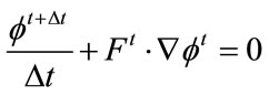
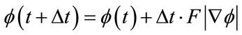
Equation (1), the level set equation, needs to be discretized for computation. This is done using the up-wind differencing scheme [31].
A first order accurate method for time discretization of Equation (1), is given by the forward Euler method, from [31]:
 (9)
(9)
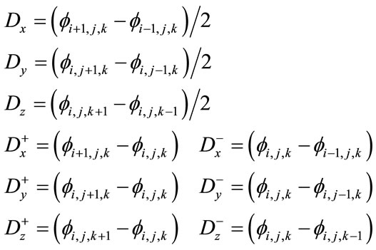
A process of choosing which approximation for the spatial derivative of  to use based on the sign of F that is known as upwinding. Results in the derivatives below required for the level set equation update [32].
 (10)
(10)
 is approximated using the upwind scheme.
 (11)
(11)
 (12)
(12)
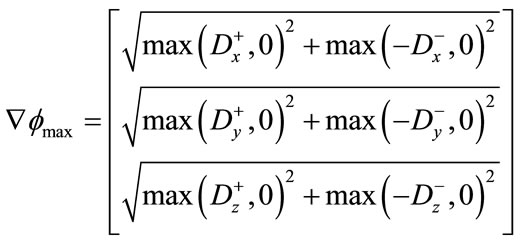
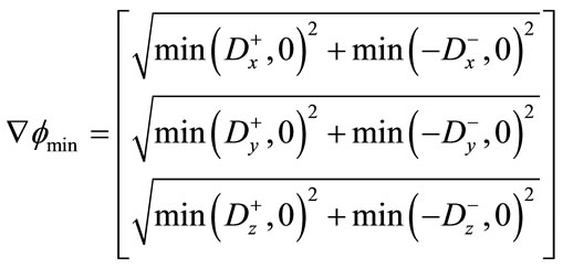
Finally, depending on whether 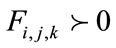 or
or 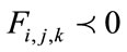 ,
,  is
is
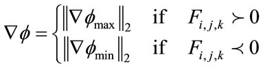 (13)
(13)
 (14)
(14)
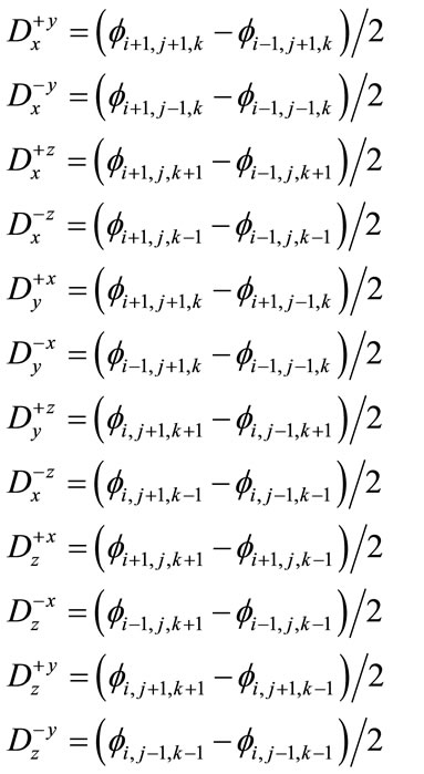
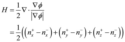
1.2. Curvature
Curvature is computed based on the values of the current level set using the derivatives below.
 (15)
(15)
Using the difference of normals method from [32], curvature is computed using the above derivatives with the two normals  and
and .
.
 (16)
(16)
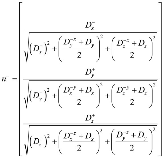 (17)
(17)
The two normals are used to compute divergence, allowing for mean curvature to be computed as shown below in Equation (12).
 (18)
(18)
1.3. Stability
Stability is enforced using the Courant-Friedrichs-Lewy (CFL) condition which states the numerical wave speed must be greater than the physical wave speed.
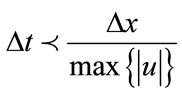 (19)
(19)
where  are the
  components of
 .
.
1.4. Level Set Implementation
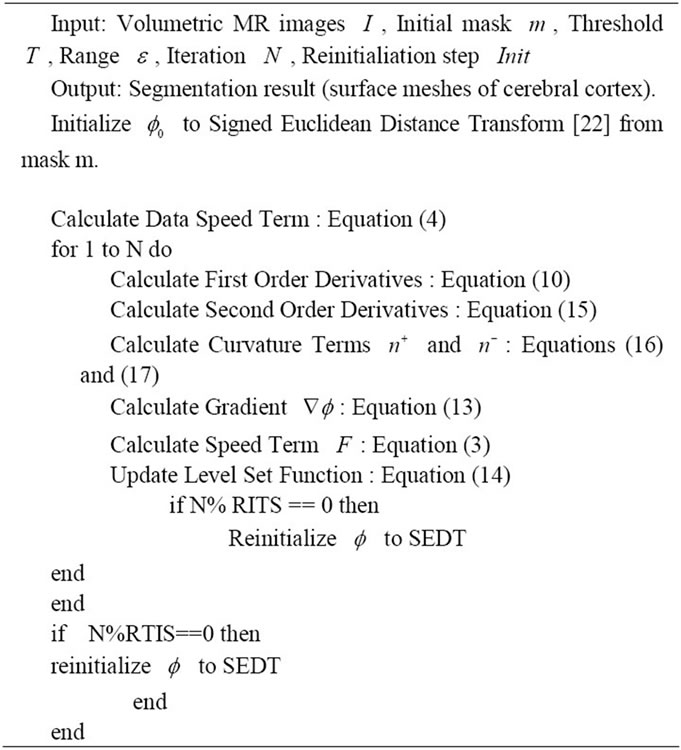
The following pseudo code outlines the structure of the level set algorithm implementations:
NOTES
*Corresponding author.