International Journal of Geosciences
Vol.4 No.1(2013), Article ID:27025,10 pages DOI:10.4236/ijg.2013.41010
Adjustment of Gravity Observations towards a Microgal Precision
1Universidade do Estado do Rio de Janeiro, Rio de Janeiro, Brazil
2Observatório Nacional/MCTI, Rio de Janeiro, Brazil
3Instituto Federal Fluminense, Itaperuna, Brazil
Email: *francismar@on.br, *francismarrb@yahoo.com.br
Received September 30, 2012; revised October 26, 2012; accepted November 28, 2012
Keywords: Calibration; Gravimeter; Gravity Network; Adjustment; Modeling
ABSTRACT
Gravity observations adjustment is studied having in view to take full advantage of the modern technology of gravity measurement. We present here results of a test performed with the mathematical model proposed by our group, on the adjustment of gravity observations carried out on network design. Additionally, considering the recent improvement on instrumental technology in gravimetry, that model was modified to take into account possible nonlinear local datum scale factors, in a 1900 mGal range network, and to check its significance for microgal precision measurements. The data set of the Brazilian Fundamental Gravity Network was used as case study. With about 1900 mGal gravity range and 11 control stations the Brazilian Fundamental Gravity Network (BFGN) was used as case study. It was established mainly with the use of LaCoste & Romberg, model G, gravimeters and new additional observations with Scintrex CG-5 gravimeters. The observables involved in the model are instrumental reading, calibration functions of the gravimeters used and the absolute gravity values at the control stations. Gravity values at the gravity stations and local datum scale factors for each gravimeter were determined by least square method. The results indicate good adaptation of the tested model to network adjustments. The gravity value in the IFE-172 control station, located in Santa Maria, had the largest estimated correction of −10.4 µGal (1 µGal = 10 nm/s2), and the largest residual for an observed reading was estimated in 0.043 reading unit. The largest correction to the calibration functions was estimated in 6.9 × 10⁻⁶ mGal/reading unit.
1. Introduction
Gravimetry has experienced an important development, in both absolute and relative measurement technique. The modern gravimeters allows observations with some microgals of precision (1 microgal = 10 nm/s2), which means an improvement of at least one order of magnitude in comparison with previous instruments. This fact suggests a review in the technical processing of gravimetric observations, in order to fully explore the modern instrumental technology. This caution is especially appropriate when the points of observation are designed in network structure for reference to future surveys. In this case, the quality of results should be the best possible, ensuring high precision and homogeneity in the gravity values of the network. Therefore, the observations involve, necessarily, the superabundant data acquisition, using two or more instruments. This implies the need for adjustment of observations with appropriate mathematical model and constraints to compensate ambiguities.
Dias and Escobar [1] proposed a mathematical model for adjustment of differential gravity measurements, involving simultaneously gravity values, coefficients of the calibration functions and instrumental readings, here named D & E model. Considering the recent development technological instrumental in gravimetry, the goal of this work is testing and improvement of the D & E model for its application in adjustments of reference gravity networks.
2. The Data Set: Brazilian Fundamental Gravity Network
Figure 1 shows the distribution of the Brazilian Fundamental Gravity Network (BFGN) stations [2]. The network involves 1739 observations of 639 gravity intervals, on 534 gravity stations, including 11 control stations. Gravity intervals were measured using 16 LaCoste & Romberg (LCR), model G, gravimeters and 5 Scintrex CG5 (CG5) gravimeters. Table 1 shows the number of observation performed with each instrument. Gravity values on control stations were measured with a free fall
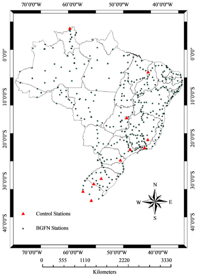
Figure 1. The 534 gravity stations of the BFGN.
gravimeter JILAG-3, with an estimated accuracy better than 10 µGal [3] (Table 2). The observations on Gravity Calibration Line Observatório Nacional-Agulhas Negras, GCLONAN [4,5] were inserted in data set of the BFGN to enhance the control of the scales of the instruments in the adjustment [6-8]. This GCLONAN (Figure 2) is composed by 13 gravity stations with a gravity range of 628 mGal, subdivided in 12 intervals. The distance is about 250 km long with an altitude variation of 2.50 km. The Table 3 shows the values of gravity intervals between stations.
3. Effects on Gravity Measurements
The instrumental readings on a same station aren’t constants. More notables variations are Earth tides and instrumental drift effects. Earth tides are related to the gravitational interaction between Earth and others celestial bodies, mainly the Moon and the Sun, they cause periodic variations as their positions change, it is a time-dependent function. Logman’s formulas [9] were used to perform Earth tides corrections. The instrumental drift is inherent to gravimeters. It is a slow and progressive variation with the time [6,10]. The drift rate depends on the conditions which the gravimeter is submitted [11,12]. The better procedure is to assume a drift rate for each gravity interval, removing the drift prior to the adjustment to avoid an over parameterization in processing.
When a CG5 gravimeter is used, the tripod is absolutely necessary to make measurements. The sensor of the gravimeter is at a specific height (Δh) from the ground (Figure 3) [13,14]. So, it is necessary to apply a correction  related to Δh, given by:
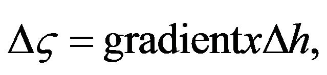 (1)
(1)
Table 1. Statistic of the gravimeters used in the BFGN.
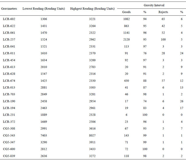
Table 2. Absolute gravity values in the control stations.
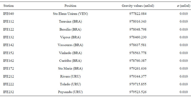
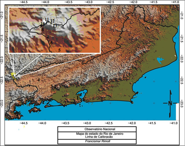
Figure 2. Thirteen gravity stations of the GCLONAN: 1—Rio de Janeiro “C”; 2—Paracambi1/4; 3—Obelisco da Serra; 4—Barra Mansa; 5—Engenheiro Passos; 6—CAL2-1; 7—CAL2-2; 8—Fazenda Lapa; 9—Marco Zero; 10—CAL4-2; 11— CAL4-4; 12—CAL4-5; 13—Posto do Ibama.
Table 3. Positioning of the gravity stations in the ONANGCL.
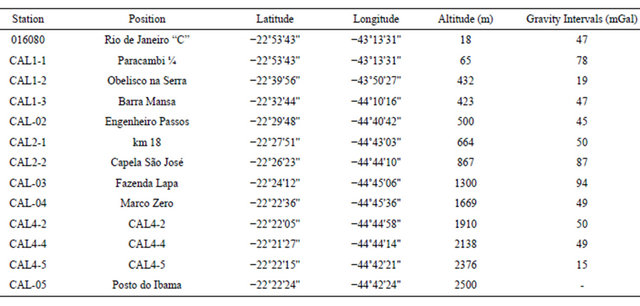
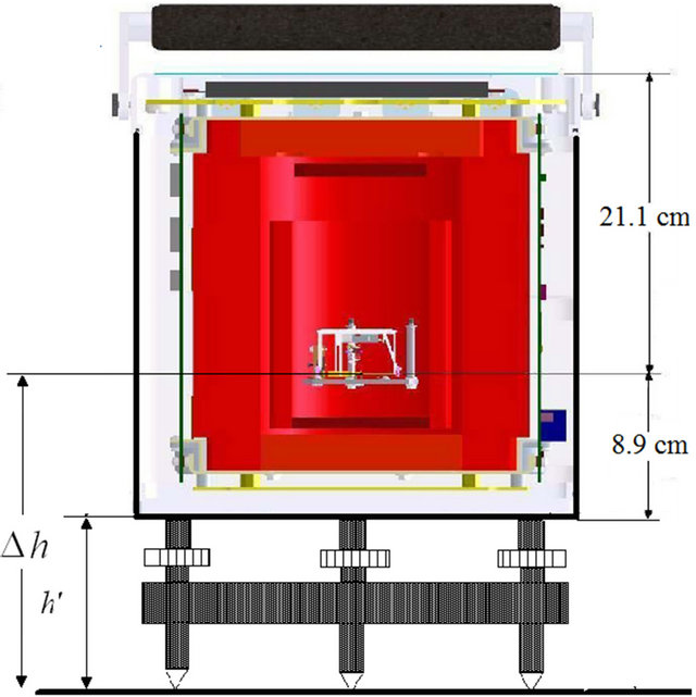
Figure 3. CG5 gravimeter scheme.
The value of the height  is measured by the operator before starting the measurements, in cm. Local vertical gradients on the stations are measured with the CG5 gravimeters by the operator.
The variations in pressure, temperature, magnetization, groundwater mass and atmospheric mass were not considered in this work for the following reasons: 1) The modern gravimeters are provided with a device for compensation of the internal pressure variation and are sealed to reduce the effects of the atmospheric pressure variation, 2) The instrumental readings were not corrected of the temperature effect, since the gravimeter has a thermostatic control device, 3) The gravimeters are submitted to the demagnetization during your manufacture and 4) The gravity change due to variation in groundwater mass were not considered by the difficulty on obtaining adequate data to determine the influence on the relative measurements of gravity in different locals. For the same reason, the influence of the atmospheric mass was not considered.
4. The D & E Mathematical Model
The D & E model [1,15] is a linear mathematical model, applicable to any differential gravimeter. It involves coefficients of the calibration functions of the gravimeters (αi), unknown, or adjusted, gravity values (gi), linear scale factors, related to the local datum, for each gravimeter (kr), and instrumental readings (li). Nonlinear calibration functions of the gravimeters are assumed. For LCR gravimeters, they are provided by manufacturer as tables that discretize them in linear intervals of 100 to 100 units and, for CG5, as a constant factor, equal to unit, which can be attributed for all discretized intervals. The mathematical model is:
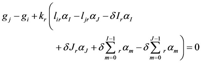 (2)
(2)
where r indicates the gravimeter used in measurements, I is an integer number equal to the number of discretization intervals embraced by
 J is analogous to I for the reading lj, δ is the interval used for the discretization of the calibration function.
The solution of this model by the least square method requires the a priori knowledge of gravity values in at least two control stations. These values were introduced as relative constraints, weighted according to the inverse of their estimated variances, with an additional model [16]:
 (3)
(3)
where ![]() represents the absolutes gravity observations on the control stations, and g is the same as in Equation (2).
represents the absolutes gravity observations on the control stations, and g is the same as in Equation (2).
In this paper, the observables were weighted according to the inverse of their variances having in view that they are of different precisions: 1) for the instrumental readings, the standard deviation was estimated equal 0.025 RU1, for LCR gravimeters, and 0.010 RU, for CG5 gravimeters. The inverse of their variance was multiplied by the number of observations performed for the gravity interval, 2) there is no explicit indication of the precision for coefficients of calibration functions of gravimeters. However, truncation in the calibration table of LCR gravimeters suggests a standard deviation equal 10−5 mGal/ RU 3) for absolute gravity values were used the standard deviation listed in Table 2. The a priori variance  of the weight unit was assumed to be equal to 1.
5. Results of the Application of the D & E Model
Solving Equation (2) by the Least Square Method (LSM), the variance of the weight unit estimated a posteriori is given by:
 (4)
(4)
where ![]() is the array of residuals, P is a weight coefficient matrix for the observables, and n is the degree of freedom for the adjustment.
is the array of residuals, P is a weight coefficient matrix for the observables, and n is the degree of freedom for the adjustment.
The estimated value for a posteriori variance of the weight unit was found equal to 1.01, which is close to the unit, a priori value assumed, which shows the consistency of the weight coefficient matrix (P).
The largest residual found for the gravity values on the control stations was −10.4 µGal, at the station IFE172, which is less than twice the estimated standard deviation for the gravity values on control stations (18 µGal). Table 4 and Figure 4 show adjusted gravity values and residuals estimated on control stations.
The largest residual for the instrumental readings was 0.043 RU, that is less than twice of the estimated standard deviation of the readings initially established (2σl = 0.050 RU). The distribution of the residuals for adjusted instrumental readings is given in Figure 5.
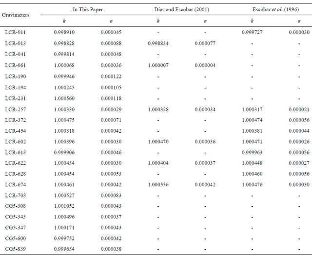
Local datum scale factors for each gravimeter were estimated as unknown parameters with good agreement with those obtained previously by [1] and [4], see Table 5. The standard deviations, σk, are related to the number of observations carried with the correspondent instrument. The greater the number of observations better tends to be the estimated standard deviation. The LCR gravimeter G257, with 2120 observed gravity intervals (Table 1), shows better standard deviation than others gravimeters, while for instruments G190, G194 and G231 the estimated standard deviations are worst. The Scintrex CG5-343 with 144 observed gravity intervals, shows better standard deviation than others Scintrex CG5 gravimeters, which show better quality than LCR gravimeters, even with fewer observations than those.
As shown, the D & E model applied in this paper also allows corrections to the coefficients of the calibration
Table 4. Adjusted gravity values and their standard deviations on control stations.
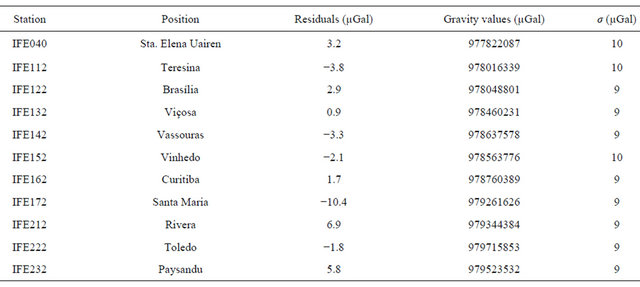

Figure 4. Residuals estimated in gravity values on control stations, by the application of D & E model.
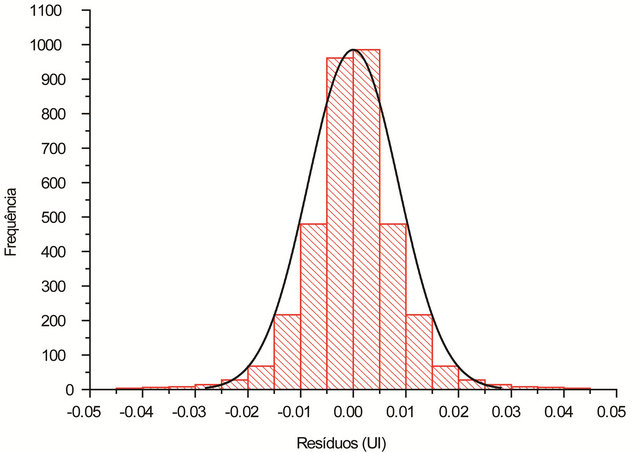
Figure 5. Histogram of residuals for adjusted instrumental readings, by the application of D & E model. In black, Gaussian curve, with the same mean value and standard deviation (0.000 ± 0.009 RU).
Table 5. Local datum scale factors for each gravimeter estimated in the adjustment.
functions to each gravimeter [1,15]. The largest residual for adjusted coefficients was found as 0.0000069 mGal/ RU, which is smaller than the standard deviation used in weighting of those parameters and is statistically insignificant.
6. The Improvement of the D & E Mathematical Model
Verified the viability of applying the D & E model in the network adjustment, a change in the D & E model was carried out to evaluate its suitability to modern gravimeters, which has a microgal reading resolution, like a Scintrex CG-5. One aspect to be explored refers to the correction to local gravimetric datum, which normally is done by linear scale factors, kr, applied to the entire scale range of each gravimeter. The improvement includes the removal of linear scale factors in the Equation (2) and the insertion of scale factors for local datum by intervals in the calibration tables of gravimeters,  , as in Equation (5). These factors by intervals provide the homogenization of the scales of the instruments, both to the local datum and among themselves, and will be determined as unknown parameters in the gravity network adjustment by the least-squares method.
 (5)
(5)
Values of kr, determined in the previous adjustment with D & E model, Table 5, was used as approximated values for scale factors by intervals, . Then, values of
  are introduced as relative constraints, weighted according to the inverse of their estimated variances, as they were determined in the previous adjustment. The additional constraint equations, to be included in Equations (3), are of the type:
 (6)
(6)
7. Application of the Improved D & E Mathematical Model
In the Equation (5), unknown parameters are the gravity values on network stations (gi) and residual scale factors for intervals ; the observables are instrumental readings (li), absolute gravity values on control stations
  , introduced by a constraint model (Equation (3)), and the approximated values for local datum scale factors for intervals
 , introduced by a constraint model (Equation (6)).
The estimated value for a posteriori variance of the weight unit was found equal to 1.009, which is close to the unit, a priori value assumed, which is an evidence of the consistency of the weight matrix (P).
The largest residual found for the gravity values on the control stations was −11.2 µGal, at the station IFE172, which is less than twice the estimated standard deviation for the gravity values on control stations (16 µGal). The Table 6 shows adjusted gravity values and residuals estimated on control stations with the improved D & E mathematical model.
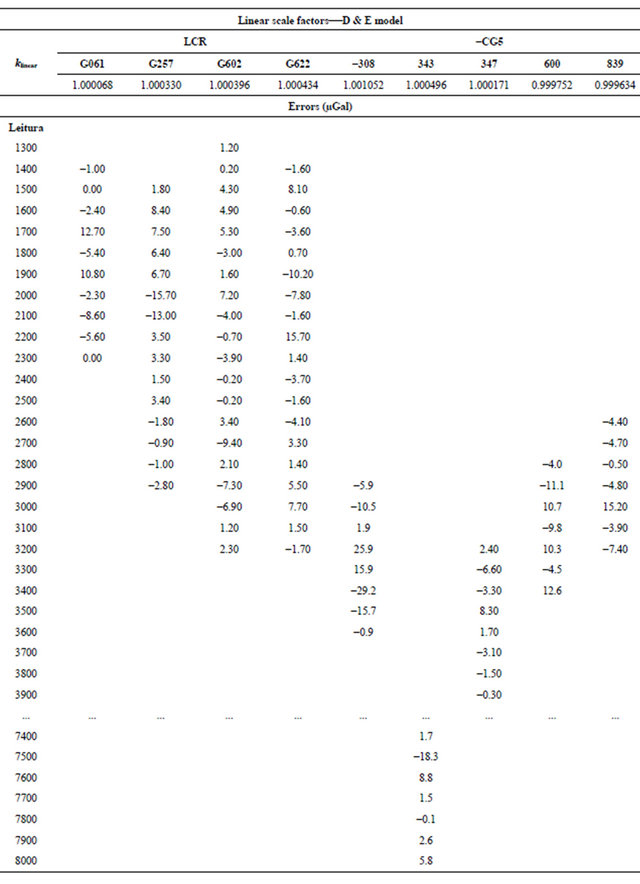
The Table 7 shows the differences among linear factors and factors by intervals, multiplied by 100 RU, which is the discretization interval adopted to the calibration table. For the LCR gravimeter, G257, a reading in the interval 2000 would be subject to an error of −15.7 microgal. For CG5 gravimeters, the large value for the error was −29.2 µGal found in instrument 308, in the interval 3400. Values in the same order of magnitude are observed to others gravimeters. For some gravimeters, with few observations, errors seem to have no statistical significance.
Table 6. Adjusted gravity values and their standard deviations on control stations.
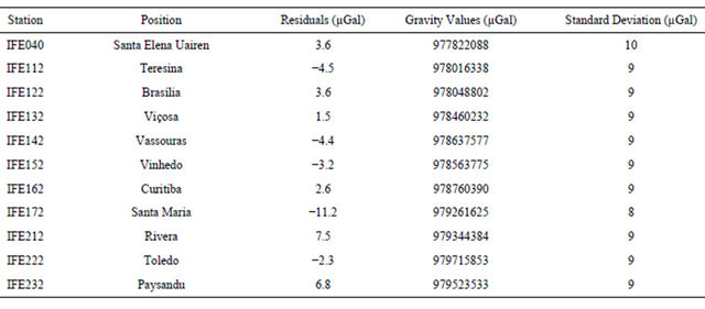
Table 7. Errors associated in the intervals.
8. Conclusions
The D & E model was used to provide appropriate adjustment of gravity network (see Figures 4 and 5). Beyond of gravity values estimation, it was used to estimate values for local datum scale factors, in a linear approach (Table 5), which was used as input in an adjustment with an improved model (Equation (5)) to evaluate its nonlinearity.
When a microgal precision is required, the improved model reveals significant nonlinearity in local datum scale factors, for the reading range of about 2000 mGal, as that found in the BGFN, see Table 7. For LCR gravimeters the larger nonlinearity error of −15.7 µGal was estimated in the reading interval around 2000 RU of the instrument G257, for CG5 gravimeters, the larger nonlinearity error of −29.2 µGal was estimated in the reading interval around 3400 RU of the instrument 308.
Weights based in the estimated standard deviations seem to be adequate (0.025 RU for LCR instrumental readings, 0.010 RU for Scintrex CG5 instrumental readings, 1 × 10⁻⁴ mGal/RU for preliminary local datum scale factors and values presented in Table 2 for control stations). The a posteriori variance of the weight unit was estimated close to the unit (1.009 mGal2), which is the expected value due to the weighting criteria used.
All estimated residuals for observables were found less than two times the respective standard deviations. No systematic effect was observed in the distribution of estimated residuals for observables.
9. Acknowledgements
I. P. E. acknowledge partial financial support from the Brazilian Sciences Funding Agency FINEP. F. R. B. thanks a Ph.D. fellowship from the Brazilian Education Funding Agency CAPES and, finally, A. R. R. P. acknowledge partial financial support from the Brazilian Sciences Funding Agencies FAPERJ and CNPq.
REFERENCES
- F. J. S. S. Dias and I. P. Escobar, “A Model for Adjustment of Differential Gravity Measurements with Simultaneous Gravimeters Calibration,” Journal of Geodesy, Vol. 75, No. 2, 2001, pp. 151-156. doi:10.1007/s001900100168
- I. P. Escobar, “Rede Gravimétrica Fundamental Brasileira, uma Tradição de 10 anos no Observatório Nacional,” Revista Geofísica IPGH, Vol. 26, 1987.
- W. Torge, L. Timmen, R. H. Roder and M. Schnull, “The IFE Absolute Gravity Program South America 1988- 1991,” Deutsche Geodatische Kommission, Munchen, 1994.
- I. P. Escobar, N. C. Sá, J. J. Dantas and F. J. S. S. Dias, “The Observatório Nacional Agulhas Negras Gravity Calibration Line,” Brazilian Journal of Geophysics, Vol. 14, No. 1, 1996, pp. 59-68.
- M. A. Sousa and A. A. Santos, “Absolute Gravimetry on the Agulhas Negras Calibration Line,” Revista Brasileira de Geofísica, Vol. 28, No. 2, 2010, pp. 165-174. doi:10.1590/S0102-261X2010000200002
- E. Parseliunas, P. Petroskevicius, R. Birvydiene and R. Obuchovski, “Investigation of the Automatic Gravimeters Scintrex CG-5 and Analysis of Gravimetric Measurements,” The 8th International Conference, Vilnius, 19-20 May 2011.
- T. Oja, T. Nikolenko, K. Türk, A. Ellmann and H. Jürgenson, “Calibration Results of Different Type Spring Gravimeters from the Repeated Measurements of Estonian Calibration Line,” NKG General Assembly, 2010.
- T. Oja, T. Nikolenko, K. Türk, A. Ellmann and H. Jürgenson, “Analysis of Gravimetric Observations Made by Scintrex CG-5,” The 7th International Conference, Vilnius, 22-23 May 2008.
- I. M. Longman, “Formulas for Computing the Tide Acceleration Due to the Moon and the Sun,” Journal of Geophysical Research, Vol. 64, No. 12, 1959, pp. 2351-2356. doi:10.1029/JZ064i012p02351
- LaCoste & Romberg, “Instruction Manual Model G&D Gravity Meters,” Austin, 2004.
- C. H. Angus and B. G. Brulé, “Vibration-Induced Drift in LaCoste & Romberg Geodetic Gravimeters,” Journal of Geophysics Research, Vol. 72, No. 8, 1967, pp. 2187- 2197. doi:10.1029/JZ072i008p02187
- V. D. Yushkin, “Operating Experience with CG5 Gravimeters,” Measurement Techniques, Vol. 54, No. 5, 2011, pp. 486-489. doi:10.1007/s11018-011-9753-5
- SCINTREX, “CG-5 Scintrex Autograv System Operation Manual,” Revision 7, Canada, 2010.
- M. Lederer, “Accuracy of the Relative Gravity Measurement,” Acta Geodynamica et Geomaterialia, Vol. 6, No. 3, 2009, pp. 383-390.
- F. J. S. S. Dias, “Um Modelo Matemático para Ajustamento Gravimétrico com Aprimoramento das Funções de Calibração dos Gravímetros LaCoste & Romberg,” MSc. Thesis, Observatório Nacional, Rio de Janeiro, 1997.
- I. P. Escobar “Injunções Relativas em Ajustamento Gravimétrico,” Publicação do Observatório Nacional, MSc Thesis, UFPR, Curitiba, No. 2, 1998.
NOTES
*Corresponding author.
1Reading Unit.