American Journal of Climate Change
Vol.05 No.02(2016), Article ID:67809,14 pages
10.4236/ajcc.2016.52022
Oceanic Indices for Forecasting Seasonal Rainfall over the Northern Part of Brazilian Northeast
Gbèkpo Aubains Hounsou-Gbo1,2,3*, Jacques Servain4,5, Moacyr Araujo1,2, Eduardo Sávio Martins6, Bernard Bourlès3,7, Guy Caniaux8
1Laboratório de Oceanografia Física Estuarina e Costeira (LOFEC), Departamento de Oceanografia da Universidade Federal de Pernambuco (DOCEAN-UFPE), Recife, Brazil
2Rede Brasileira de Pesquisas sobre Mudanças Climáticas Globais (Rede Clima), São José dos Campos, Brazil
3International Chair in Mathematical Physics and Applications (ICMPA), UNESCO Chair, Cotonou, Benin
4Institut de Recherche pour le Développement (IRD), LOCEAN, Paris, France
5Departamento de Oceanografia, UFPE, Recife, Brazil
6Fundação Cearense de Meteorologia e Recursos Hidricos (FUNCEME), Fortaleza, Brazil
7Institut de Recherche pour le Développement (IRD), LEGOS, Brest, France
8CNRM UMR 3589, Météo-France/CNRS, Toulouse, France

Copyright © 2016 by authors and Scientific Research Publishing Inc.
This work is licensed under the Creative Commons Attribution International License (CC BY).
http://creativecommons.org/licenses/by/4.0/


Received 29 December 2015; accepted 25 June 2016; published 29 June 2016
ABSTRACT
A relationship between oceanic conditions in the northwestern equatorial Atlantic (NWEA) and the seasonal rainfall over the northern part of Brazilian Northeast (NNEB) allows large climate events to be forecasted with a delay of a few months. Observed sea surface variables (sea surface temperature, wind stress and latent heat flux) and reanalyzed temperature and salinity profiles at depths of 0 - 150 m are used during 1974-2008. Perturbations in the Wind-Evaporation-SST mechanism over the NWEA during the last months of the year and the first months of the following year are of primary importance in evaluating the risk that strong climate events will affect the subsequent seasonal rainfall (in March-April) over the NNEB. Especially interesting are the Barrier Layer Thickness (BLT) and Ocean Heat Content (OHC) in the NWEA region from August-Sep- tember through the subsequent months, during which a slow and steady evolution is apparent, with the highest signal occurring in October-November. Through their relationship with the local surface dynamic conditions, such BLT and OHC perturbations during the last months of the year can be used as a valuable indicator for forecasting wet or dry events over the NNEB during the subsequent rainfall season. A proposal is discussed to deploy additional temperature/conducti- vity sensors down to a depth of 140 m at three PIRATA moorings located in the NWEA region. That will be necessary if the BLT and other parameters of energy exchange between the ocean and atmosphere are to be estimated in real time and with a sufficiently high vertical resolution.
Keywords:
Brazilian Northeast, Seasonal Rainfall, Barrier Layer Thickness, Oceanic Heat Content

1. Introduction
Except along the coast, the climate of the Brazilian Northeast (NEB; locally called “Nordeste”) is largely semiarid, with notable seasonal and interannual variability in rainfall. Exceptionally wet or dry episodes are often associated with worldwide and regional climate phenomena, such as El Niño-La Niña episodes [1] [2] or the formation of a meridional Sea Surface Temperature (SST) gradient over the tropical Atlantic [2] - [7] .
During El Niño episodes, there is a tendency toward the inhibition of convective activity over the western tropical Atlantic, which is associated with predominantly weak precipitation, off the northern coast of the NEB [8] [9] . Conversely, during La Niña occurrences, there is frequent reinforcement of westward convective systems over that region, which is favorable to increased precipitation over the NEB.
During a typical negative phase of the meridional SST gradient, which is characterized by a negative SST anomaly and enhanced evaporation in the northern tropical Atlantic, and also a positive SST anomaly and less evaporation in the south, the thermal gradient is directed toward the Southern Hemisphere [10] . Consequently, the intertropical convergence zone (ITCZ)―characterized by a high degree of cloudiness and huge amounts of precipitation―is predominantly located to the south of its climatological position. This generally leads to more rain over the NEB, especially in the northern subregion [3] [4] [11] . Conversely, during a positive phase of the meridional SST gradient, the ITCZ moves northward from its climatological position and precipitation rates are generally below average in the NEB. In some instances, these changes lead to dramatic dry episodes in the region. [10] interpreted this ocean-atmosphere relationship in the tropical Atlantic basin as a positive feedback phenomenon linked to the Wind-Evaporation-SST (WES) mechanism that sustained the meridional SST gradient.
Based on data from the second half of the Twentieth Century, [12] reported that the climatic impact related with the tropical Atlantic itself seemed significantly more consistent than that directly linked to El Niño-La Niña episodes. In fact, the primary reason for wet or dry episodes in the NEB is the development of negative or positive meridional gradient patterns. Except for very strong El Niño or La Niña episodes, the Pacific influence is only a secondary contributor to rainfall variability. Additional reasons for the seasonal rainfall variability in the NEB are related to deep convection, atmospheric instability lines, breeze occurrences, and atmospheric easterly waves.
Precise operational monitoring of surface conditions (SST, wind, evaporation, etc.) in the most sensitive ocean areas as related to precipitation over the NEB is thus of paramount importance for understanding and predicting potential major events during the coming rainy season in this region. This effort is the main objective of the present study, which is an extension of a recently published article by Hounsou-Gbo et al. [13] , in which abnormal surface and subsurface conditions in the tropical Atlantic are shown to have a valuable relationship with the subsequent seasonal rainfall over two subregions of the NEB. The present study focuses on one of these subregions, the northern part of NEB, hereafter referred to as the NNEB. The peak of the rainfall season in the NNEB, which is statistically well represented by data from the meteorological station at Fortaleza, Ceará (See Hounsou-Gbo et al. [13] ), occurs during the March-April period (hereafter MA). The low-frequency variability of meteo-oceanic information collected over the northwestern region of the equatorial Atlantic (NWEA), is analyzed here to forecast seasonal rainfall in the NNEB a few months in advance.
After a brief description of the data used and the method of analysis applied (Section 2), in Section 3, we enlarge on several main results of Hounsou-Gbo et al. [13] that are fundamentally associated with the relationship between oceanic conditions in the NWEA and the subsequent rainfall season over the NNEB. In Section 4, we focus on the oceanic potential to predict the intensity of the seasonal rainfall in the NNEB. Finally, a technical solution for the implementation of a warning system for strong wet or dry March-April events in the NNEB region is proposed in the final section. This solution is based on achieving a higher vertical resolution for real-time observations of temperature and salinity at three “Prediction and Research Moored Array in the Tropical Atlantic” (PIRATA) buoys located in the NWEA [14] [15] .
2. Data and Method
The observed and simulated data used here are partially the same as those used by Hounsou-Gbo et al. [13] . Because of the unavoidable homogeneity in the different jointly analyzed data bases, the study period is limited to 1974-2008 (35 years), with a monthly temporal resolution. The precipitation data set is composed of rainfall observations measured at a meteorological station at Fortaleza, Ceará (03˚43S; 38˚32W). It has been proven (not shown here) that these data, obtained from the Fundação Cearense de Meteorologia e Recursos Hídricos- FUNCEME (http://www.funceme.br), are representative (COR = 0.88) of the average precipitation over the entire NNEB (03˚S to 05˚S; 43˚W to 38˚W). In the following, any mention of precipitation at Fortaleza or in the NNEB should be taken to refer to the same variable. From the 35 years of the study period, Hounsou-Gbo et al. [13] selected 20 years with strong rainfall events (absolute value >0.5 STD) during MA. Among these 20 episodes, 8 were characterized as very wet (1974, 1985, 1986, 1991, 1995, 1996, 2001, and 2003), whereas 12 were very dry (1977, 1978, 1979, 1980, 1982, 1983, 1990, 1992, 1993, 1998, 2005, and 2006).
All meteorological and oceanic data sets used here provide data on the tropical Atlantic (20˚N to 20˚S), with various spatial resolutions. Monthly pseudo-wind stress (PWS) vectors, with a 2˚ × 2˚ resolution, were obtained from the Servain data set [16] [17] , which is routinely processed at FUNCEME from individual World Meteorological Office (WMO) Voluntary Observing Ship (VOS) reports, buoy measurements (including the PIRATA network) and other in situ Ocean Data Acquisition Systems (ODASs). Monthly observed SST and latent heat flux (LHF) data, with a 1˚ × 1˚ resolution, were obtained from the Objectively Analyzed air-sea Fluxes Project (OAFlux) [18] and are available from the Woods Hole Oceanographic Institution (WHOI) (http://oaflux.whoi.edu).
Simulated oceanic temperature and salinity data were obtained from the Simple Ocean Data Assimilation (SODA) [19] available at http://iridl.ldeo.columbia.edu, with a 0.5˚ × 0.5˚ horizontal resolution. The SODA reanalysis is vertically distributed in 40 levels, from 5 m to 5375 m, with 10 m spacing in the top layer. These subsurface data, linearly and vertically interpolated to 1 m spacing in the top layer, are used to determine the monthly isothermal layer depth (ILD) and the density mixed layer depth (MLD). In the present study, using the criterion  [20] , the ILD corresponds to the depth at which the temperature is equal to
 , where
  is the SODA temperature at reference depth
 . We consider the
  at 5 m instead of 10 m, as used by [20] for individual profiles, because of the vertical resolution of the SODA reanalysis and the characteristics of the tropical Atlantic. First, the shallowest levels of the SODA temperature and salinity profiles are situated at 5 m. Second, in the tropical Atlantic, the thermocline can sometimes be shallower than 10 m, predominantly during the boreal summer in the eastern equatorial region and especially during the cold tongue season. The MLD is determined using the density (σ) criterion with
  [20] - [22] , which is the density difference for the same change in temperature (
 ) at constant salinity.
  and
and  are the SODA temperature and salinity values, respectively, at
 , and
, and  is the pressure at the ocean surface. With this criterion, the MLD corresponds to the depth at which the potential density has increased from that at the reference depth by
 , where
  is the potential density value at the reference depth
 .
.
The MLD should be equal to the ILD for situations in which the density mixed layer coincides with the temperature mixed layer, i.e., the salinity profile remains constant within the isothermal layer. For increasing salinity (a positive vertical gradient) within the ILD, the associated increase in density induces a shallower MLD compared with the ILD. In this case, the difference between the ILD and MLD is positive and corresponds to the barrier layer thickness (BLT) [21] [22] . Otherwise, a constant density within and just below the ILD is associated with an MLD that is deeper than the ILD. This case should correspond to a negative value of the difference between the ILD and MLD, the so-called compensated layer thickness [20] .
The BLT is a characteristic of tropical ocean regions [21] , especially (1) the western tropical Pacific, (2) the eastern tropical Indian Ocean, and (3) the western tropical Atlantic, the most equatorial portion of the last- named region being our region of interest. In these three regions, a mixed layer is shallower than the isothermal layer forms, implying the presence of a halocline above the thermocline [20] [21] [23] . In the northwestern equatorial Atlantic, it is hypothesized [21] [24] that high-salinity waters are subducted in the subtropics during winter and advected westward to produce a salinity maximum in the upper layers in the tropics, resulting in the formation of barrier layers. Different possible causes contributing to the seasonal and interannual evolution of the mixed layer heat budget in the western tropical Atlantic have been proposed from observations and numerical simulations [10] [24] - [27] . For instance, [25] report that the Amazon River discharge may induce a strong halocline at depths of 3 - 30 m. It has been found [27] that seasonal variations of the BLT exert considerable influence on the SST through the modulation of the vertical heat flux at the base of the mixed layer. A thick barrier layer (BL) suppresses/reduces the upward transfer of cold water from the upper thermocline into the mixed layer. Consequently, a thick BL is associated with a warm SST [27] , whereas the presence of a thin or inexistent BL enhances SST cooling.
The SODA temperature profiles are also used to determine the ocean heat content (OHC, expressed in GJ m−2), from the vertical integration of the temperature within the ILD. OHC is an important parameter for quantifying the amount of upper oceanic heat that directly interacts with the surrounding atmosphere through energy and mass transfer.
3. The WES Mechanism and the Seasonal Rainfall in the NNEB
Hounsou-Gbo et al. [13] analyzed the spatio-temporal evolution of various oceanic variables in the tropical Atlantic a few months prior to the peak of the rainfall season in the NNEB, which occurs in MA. Here, Figure 1 shows five additional patterns of linear regression coefficients between LHF (shaded regions) and PWS (vectors) anomalies over the entire tropical Atlantic, and rainfall anomalies at Fortaleza. The linear regressions, averaged over 2 months, were computed using only the 20 years during the period 1974-2008 that corresponded to strong rainfall variability (either > +0.5 STD or < −0.5 STD) at Fortaleza. The five patterns in Figure 1 are related to the regressions of LHF and PWS anomalies during the bimonthly periods ND, DJ, JF, FM and MA with respect to the rainfall anomalies during MA at Fortaleza. The linear regression at zero lag (i.e., during MA) exhibits an obvious meridional dipole pattern for LHF and PWS. A strong positive relationship of rainfall anomalies with LHF (i.e., increased evaporation, up to 14 mm month−1 W−1 m−2) is observed in the west between 10° N and the equator, and a negative relationship (down to −14 mm month−1 W−1 m−2) is observed in a zonal region immediately south of the equator. This meridional pattern of LHF anomalies is intimately related to a meridional dipole in the wind stress perturbation. The high positive coefficients of the linear regression in the northern part of the dipole between the LHF and rainfall at Fortaleza are associated with an acceleration of the northeasterly trade winds in this region. Conversely, the high negative values of the LHF and rainfall regressions are associated with a relaxation of the southeasterly trade winds in the southern part of the dipole. Such LHF and PWS patterns agree quite well with the positive impact of the meridional SST gradient on the rainfall variability in the NNEB [4] [5] , which has already been widely discussed in the literature (cold SST in the North, warm SST in the South) and is fully illustrated in Figure 4 of Hounsou-Gbo et al. [13] . The WES mechanism [10] , which relies, in an anti-symmetrical manner on either side of the equator, on the strengthening (decrease) of the trade winds, the cooling (warming) of the SST, the occurrence of more (less) evaporation at the sea surface, and the occurrence of more (less) convective activity in the ITCZ, is fully appropriate for explaining the close relationship between the oceanic surface conditions over the western equatorial Atlantic and the occurrence of more (or less) rainfall over the NNEB. These results are in agreement with Hounsou-Gbo et al. [13] and yield further understanding of the remote dynamic processes at work. The LHF dipole gradually develops from ND (4-month lag) to MA (zero lag), the linear correlation coefficient with the MA rainfall at Fortaleza being significant from DJ, i.e., more than 2 months before the peak of the rainfall season in the NNEB. In and around the NWEA, the northeasterly trade winds and the LHF gradually increase (Figure 1), the SST gradually decreases (Figure 4 of Hounsou-Gbo et al. [13] ), and, consequently, the convective humidity transport toward the South American continent becomes gradually more intense before episodes of strong precipitation over the NNEB. The opposite oceanic conditions occur before dry episodes over the NNEB. Interestingly, three buoys of the PIRATA network (8˚N - 38˚W, 4˚N - 38˚W and 0˚N - 35˚W) are present inside the selected NWEA.
4. Subsurface Thermal Conditions in the NWEA as Precursors of the Seasonal Rainfall Variability in the NNEB
4.1 Rainfall versus PWS, SST, LHF and BLT
Hounsou-Gbo et al. [13] suggested that early knowledge of shallow oceanic conditions in the NWEA region
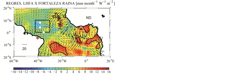
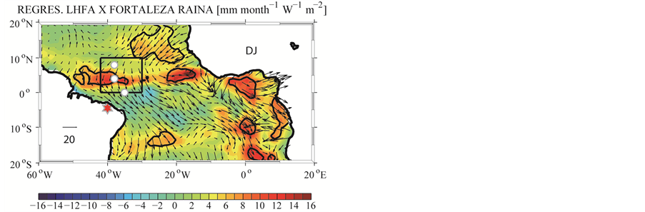
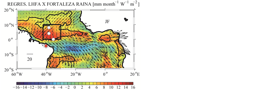
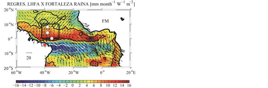
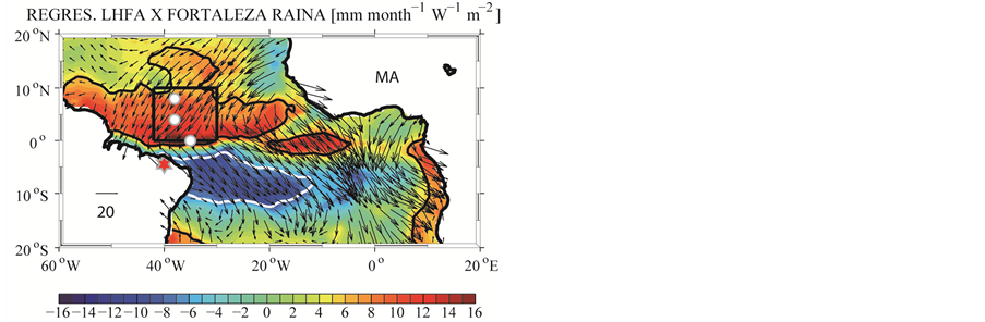
Figure 1. Distributions of lagged linear regression coefficients between the interannual rainfall anomalies in Fortaleza (red star) during March-April of the 8 wettest (>+0.5 STD) and 12 driest (<−0.5 STD) years during 1974-2008 and the interannual LHF anomalies in the tropical Atlantic for MA (zero lag), FM (1-month lag), JF (2-month lag), DJ (3-month lag), and ND (4-month lag) (mm month−1 W−1 m−2). The vectors (mm month−1 m−2 s−2) represent the linear regressions between the interannual rainfall anomalies and the interannual PWS (PWSx and PWSy) anomalies. The 95% significance level of the correlation, according to Student’s t-test (and higher than 0.5), is plotted for the LHF as a solid line (positive) and a dotted line (negative). Before averaging and plotting by 2-month periods, the linear trends were removed from all anomalies. The NWEA region (black boxes) and the positions of three PIRATA buoys (08˚N - 38˚W, 04˚N - 38˚W and 0˚N - 35˚W) are represented on the maps.
could be useful in forecasting strong precipitation anomalies in the NNEB. In the present paper, we extend this analysis, focusing on the subsurface variables: BLT and OHC. Figure 2 shows the mean annual cycles (June-to- June), averaged over 1974-2008, of five parameters. One of these parameters is the rainfall at Fortaleza, whereas the other four variables are spatially integrated over the NWEA: the meridional component of the PWS (PWSy), the SST, the LHF and the BLT. The Fortaleza MA rainfall maximum (>350 mm month−1) occurs immediately after the southward maximum of PWSy (~−37 m2 s−2, in FM), the minimum of the SST (~26.7˚C, in February),
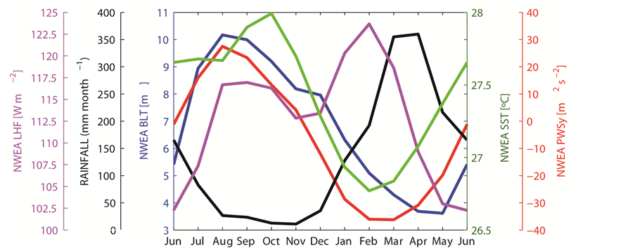
Figure 2. Seasonal climatologies (1974-2008) for the monthly rainfall at Fortaleza (mm month−1, black curve) and for four oceanic parameters averaged over the NWEA region: SST (˚C, green curve), PWSy (m2 s−2, red curve), LHF (W m−2, magenta curve) and BLT (m, blue curve).
and the second seasonal maximum of the LHF (~123 W m−2, also in February, with the LHF being positive upward). During these months, the ITCZ is at its southernmost position, i.e., close to the equator, and the convective transport of humidity in the direction of the NNEB is at its highest level. As indicated above, the progressive strengthening of the southward PWSy, the decrease of the SST and the increase of the evaporation from ND until MA beyond the climatological averages are statistically related to strong rainy events at Fortaleza. Conversely, the progressive weakening of the southward PWSy, the increase of the SST and the decrease of evaporation favor dry conditions over the NNEB during the rainy season. The beginning of the dry season (August-September) coincides with a northward PWSy and with the first maximum value of the LHF (~117 W m−2) (Figure 2). The ND period, characterized by a relative minimum in the LHF, corresponds to the transition between a northward PWSy (positive values) and a southward PWSy (negative values) in the NWEA. ND represent the period during which the ITCZ is located over the NWEA during its southward displacement. The annual cycle of the BLT (Figure 2) indicates that its highest value (~10 m) occurs in August-September and that this quantity exhibits a marked minimum in May (<4 m), i.e., at the end of the rainy season over the NNEB. Thus, a high BLT forms in the NWEA during the dry season of the NNEB (from August to December), and a low BLT is observed during the peak of the rainy season (MA). The SST minimum, in February, coincides with the maximum of the LHF, the maximum of the southward PWSy and a relatively low BLT in the NWEA. Although the seasonal minimum (maximum) of the BLT does not coincide with the minimum (maximum) of the SST, it could make a significant contribution to the seasonal cycle of the SST, as suggested by [27] .
4.2. PWS, LHF and BLT/OHC Anomalies
In the following, we present the subsurface parameters, such as the BLT and the surface layer OHC that may act as precursors of the surface oceanic and atmospheric conditions that contribute to the rainfall variability in the NNEB.
To build upon the results of Hounsou-Gbo et al. [13] regarding the forecasting of precipitation over the NNEB, we used the same methodology, jointly considering the 8 wettest years and 12 driest years (see Figure 6 of Hounsou-Gbo et al. [13] ) during 1974-2008, but now starting the study in July-August (JA), i.e., more than 8 months before the peak of the rainfall season at Fortaleza in MA. Figure 3 shows the 2-month PWSy and LHF standardized anomalies (upper panels; Figure 3(a) and Figure 3(b)), and BLT and OHC standardized anomalies (bottom panels; Figure 3(c) and Figure 3(d)) within the NWEA from JA until MA for the two series of years (wet on the left, i.e., Figure 3(a) and Figure 3(c); and dry on the right, i.e., Figure 3(b) and Figure 3(d)). All anomalies are standardized by the standard deviation of the quantity concerned for the entire period. Negative (positive) PWSy and LHF anomalies indicate a strengthening (weakening) of the PWSy component and weaker (stronger) LHFs, respectively. In the same manner, negative (positive) BLT and OHC anomalies indicate lower (higher) BLTs and smaller (larger) OHCs, respectively. The PWSy anomaly signals presented in Figure 3 exhibit a progressive variation throughout the JA-to-MA period, with larger values from JF to MA. These results show a progressive strengthening (weakening) of the PWSy component during the wettest (driest) years, the largest values of PWSy anomalies occurring only during the first months of the year, i.e., just before and during the peak of the rainy season in the NNEB. This observation confirms (as already shown in Figure 1) that the meridional wind increases (decreases) progressively from ND to MA during the wettest (driest) years, whereas the wind anomaly signal is very small or inexistent during the preceding months (i.e., July to November) for both yearly patterns. The same analysis using the LHF averaged over the NWEA area reveals a similar pattern to that of the meridional PWS but, in this case, with very strong values from JF to MA. During the wettest years, the positive LHF anomalies are very strong (>0.6 STD) from JF to MA compared with the JA-to-DJ period. For the driest years, the absolute value of the negative LHF anomalies is less (−0.5 STD) than that for the wettest years but significantly stronger than that for JA to ND. As for the meridional PWS, the stronger values of the LHF anomalies, both positive and negative, occur just before and during the peak of the rainy season.
After the evolution of the surface variables, we now present the subsurface BLT and OHC quantities. It is noticeable that, during the wettest (driest) years, large negative (positive) BLT anomalies occur from SO until ND, with a period of stronger absolute values in ON, i.e., a minimum value of about −0.6 STD and a maximum value of about +0.6 STD for the wettest and driest years, respectively (Figure 3(c) and Figure 3(d)). In ND, and during the following months (until MA), the absolute value of the BLT anomalies progressively decreases, passing through a value close to zero for both the wettest and driest years. OHC and BLT exhibit similar patterns, i.e., large negative (positive) anomalies from SO through ND for the wettest (driest) years (Figure 3(c) and Figure 3(d)). During the wettest years, the absolute value of the negative OHC anomalies decreases from a high value in SO to a small value, close to zero (~0 STD), in FM. In MA of the wettest years, the OHC anomalies exhibit a relatively positive value. For the driest years, the positive anomalies exhibit relative stability (about +0.3 STD) from JA to ND and decrease from DJ (about +0.2 STD) through MA (~0 STD).
These new results indicate that a steady, strong negative (positive) anomaly of OHC occurring during the second half of the year in the NWEA is related to strong (weak) rainfall in the NNEB during MA of the
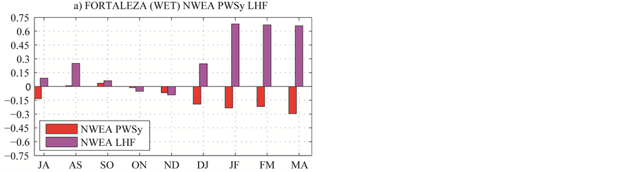
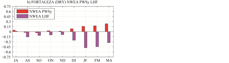
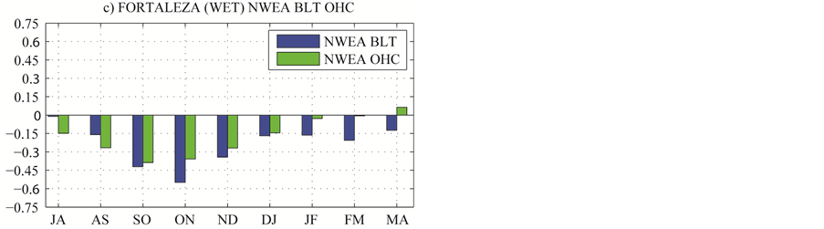
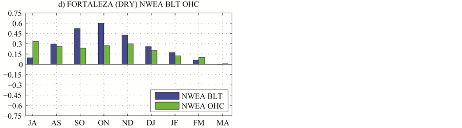
Figure 3. 2-month evolution from July-August (JA) to March-April (MA) of the standardized anomalies in the PWSy and LHF (upper panels; a and b) and in the BLT and OHC (bottom panels; c and d), averaged over the NWEA region, for the 8 wettest years (left) and the 12 driest years (right) at Fortaleza during the period of 1974-2008. Negative (positive) values of the PWSy and LHF anomalies indicate a strengthening (weakening) of the PWSy component and weaker (stronger) LHFs, respectively. Negative (positive) values of the BLT and OHC anomalies indicate lower (higher) BLTs and smaller (larger) OHCs, respectively.
following year. Our results also indicate that the presence of a steady small (steady large) BLT from SO to ND in the NWEA is related to high (low) rainfall in the NNEB during MA of the following year. Such a small (large) BLT is favorable (unfavorable) for more (less) mixing of water in the layer down to the base of the thermocline. More (less) mixing of water for a few months at the end of the year, associated with the increase (decrease) in the NE trade winds beginning in ND, leads to simultaneous cooling (warming) of the SST. In other words, it is suggested that the BLT serves as a precursor of SST cooling (or warming) by enhancing (or reducing) vertical mixing of warm surface water with the cold subsurface water at the base of the mixed layer. The combination of this BLT preconditioning with increasing (decreasing) evaporation during the first months of the subsequent year facilitates (inhibits) the convective transport of humidity in the ITCZ through the NNEB and thus increases (decreases) precipitation over the NNEB.
4.3. Spatial BLT and OHC Patterns
We now focus on the BLT and OHC patterns a few months before the rainfall season at Fortaleza at the basin scale. As a suitable example of that period, we choose the months of ON, during which the BLT anomaly signals related to both wettest and driest subsequent episodes in the NNEB are very high (see Figure 3) and which is well before the peak of the rainfall season. For conformity, we considered the same months (ON) for the OHC. In essence, ON can be regarded as an efficient period from which to obtain information on the BLT and OHC in the NWEA region while still having sufficient time to process the data to contribute to the evaluation of the subsequent seasonal rainfall forecast. The climatological patterns of the BLT (in m) and OHC (in GJ m−2) for ON averaged over the 35 years from 1974 to 2008 from the SODA data set are shown in Figure 4(a) and Figure 4(b) respectively. The limits of the NWEA are indicated, as well as the location of the three PIRATA buoys (at 8˚N - 38˚W, 4˚N - 38˚W and 0˚N - 35˚W). North of the equator, large values of BLT (>10 m) are observed in the western part of the basin, with the largest values at the mouth of the Amazon River and north of 10˚N (Figure 4(a)). Another region of thick BL is centered at 30˚W, between the equator and 10˚N. This indicates that the dynamics in this region is complex and depends on various factors (positions of the ITCZ and the North Equatorial Countercurrent, the Amazon River discharge, etc.). A weaker or inexistent BLT (<4 m) in the northern hemisphere is observed in the Gulf of Guinea and along the Mauritanian coast. South of the equator, the BLT is globally small (<4 m) or inexistent, except in the southwestern Atlantic warm pool region off Brazil. Regarding the OHC distribution, the largest values (>6.5 GJ m−2) in the northern hemisphere are located between 5˚N and the equator and also west of 30˚W, i.e., in a region where two PIRATA buoys are located, at 4˚N - 38˚W and 0˚N - 35˚W, whereas weaker OHC values (<3.5 GJ m−2) are observed close to the buoy at 8˚N - 38˚W (Figure 4(b)). Relatively strong values of OHC (~5 GJ m−2) are also observed north of 10˚N, with higher OHCs in the western region. In the southern tropical Atlantic, high OHCs are observed in the western part of the basin while the weakest OHCs are in the eastern region. The largest values of OHC (>7.5 GJ m−2), in the southern tropical Atlantic, are globally observed in the southwestern Atlantic warm pool region off Brazil. The bottom panels of Figure 4 represent the differences in ON of BLT (Figure 4(c)) and OHC (Figure 4(d)) between the two patterns corresponding to the combined values for the 12 driest years minus the combined values for the 8 wettest years considered at Fortaleza in MA. The difference is very clear in the NWEA (significant at 90% level) for both the BLT and OHC, especially from 4˚N to 8˚N. The larger values of BLT (>16 m) and OHC (>2.5 GJ m−2) differences within the NWEA are centered at 5˚N - 32˚W. Interestingly, the PIRATA buoy at 4˚N - 38˚W is located within this region of the largest differences. This indicates that there is good potential to use the PIRATA network in the region to predict climate variability over the NEB.
4.4. BLT and ILD at PIRATA Moorings
Here, we test the BLT variability at the exact geographical positions of the PIRATA buoys located in the NWEA. As an example, Figure 5 presents the results for the PIRATA buoy at 4˚N - 38˚W, where, according to Figure 4, there is a high potential to anticipate the seasonal rainfall in the NNEB. In the two top panels of Figure 5, the 0 - 150 m profiles of temperature, salinity and density are represented, together with the BLTs (shaded regions) averaged over ON and MA during the 8 wettest years in the NNEB (denoted ONW and MAW). The two bottom panels are the same but for the 12 driest years (denoted OND and MAD). Averaged over the full 35-year period (not shown), the BLT at 4˚N - 38˚W is 10 m in ON and 3 m in MA. At the sea surface, very
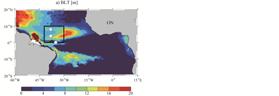
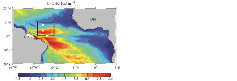
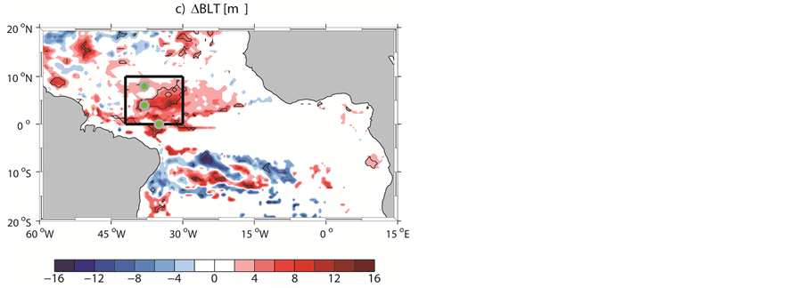
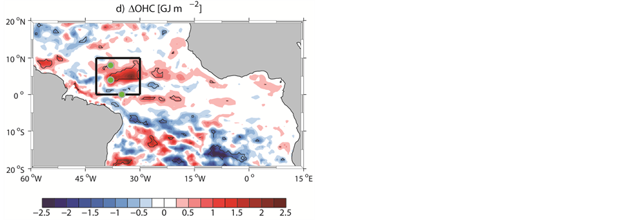
Figure 4. (Top) Climatological patterns of the BLT (m, a) and OHC (GJ m-2, b) in ON averaged over the 35 years from 1974 to 2008; (Bottom) Difference between the combinations of the data for the 12 years with the driest March-April periods and the 8 years with the wettest March-April periods at Fortaleza for the previous corresponding October-November BLT (m, c) and OHC (GJ m-2, d) patterns. Grid points where the layer thickness is less than 10% of the maximum depth (ILD or MLD) are set to zero. Contours in c and d represent regions where the differences are significant at 90% level using Welch’s t-test. The NWEA region (black box) and the locations of three PIRATA buoys are also indicated.
similar values for temperature (i.e., SST), salinity and density are observed between ONW and OND (respectively 27.8˚C, 35.8, and 23.0 kg m−3 vs. 27.7˚C, 35.8, and 23.0 kg m−3) and between MAW and MAD (respectively 27.1˚C, 35.8, and 23.2 kg m−3 vs. 27.5˚C, 35.7, and 23.0 kg m−3). Considering the vertical profiles of temperature and density between 0 and 150 m, there is very little difference between MAW and MAD and a relatively large difference between ONW and OND. These differences are mainly observed in the temperature and the density mixed layers with the IL and the ML shallower in ONW (50 m and 44 m, respectively) than in OND (65 m and 49 m, respectively). During the wettest and driest years, there is a salinity maximum at approximately 100 m in ONW and OND and at approximately 60 m in MAW and MAD, both with similar values (~35.8 vs. ~36.0). None of the values of these parameters changes significantly at the deepest levels and they exhibit similar values at 150 m, at least for the wettest years and the driest years. The vertical gradient of salinity in the halocline during the preceding ON period for the wettest years is comparable to that for the driest years (0.0017 m−1 vs. 0.0019 m−1, respectively). Although the values of the differences between the wettest and driest patterns remain low according to direct hydrographic measurements, the values deduced for BLT are clearly different. The BLT in ONW (6 m) is significantly different (95% level) from the BLT during OND, which is estimated at 16 m (Figure 5). For both the wettest and driest years, the BLT evolves toward similar values during MA (1 m and 2 m, respectively), which are not significantly different from the MA climatological mean value (3 m). The significant difference of BLT in ON between the wettest and driest years is primarily due to the difference in ILD between these years. The ILD values in ON during the wettest and driest years are 50 m and 65 m, respectively, whereas the MLD values are 44 m and 49 m, respectively. This difference in ILD between the driest and wettest
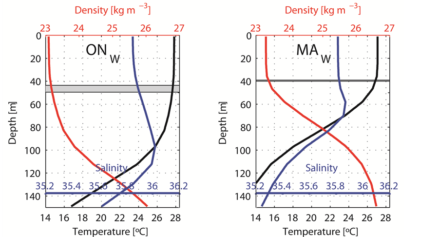
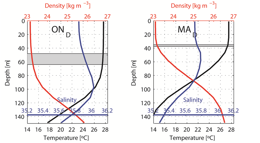
Figure 5. Vertical profiles (0 - 150 m) of temperature (˚C, black line), salinity (blue line) and density (kg m−3, red line) from SODA at the site of the PIRATA buoy at 4˚N - 38˚W, averaged over the 8 wettest years (top) and the 12 driest years (bottom) at Fortaleza during the period of 1974-2008. The profiles at the left (at the Right) are relative to the means for October-No- vember (ON) and March-April (MA), respectively. The region of the corresponding BLT values is shaded. The MLD and ILD extend from the surface to the top and bottom limits of the shaded region, respectively.
years is also associated with the strong difference in the OHC mentioned previously. The difference between the BLTs of ONW and OND (6 m vs. 16 m) suggests that suitable observations of the T/S profiles at the 4˚N - 38˚W PIRATA buoy during the last months of the year are very useful for predicting the subsequent rainfall variability over the NNEB. Obviously, to obtain an accurate rainfall forecast, such an initial indicator should be assessed in a timely manner and then followed throughout the following weeks and months through careful monitoring of other important variables (SST, wind, etc.).
5. Conclusions and Monitoring Perspectives
The present study is based on historical sea surface observations (SST, wind stress, and LHF) provided by different data sets (Servain’s data set and OAFlux) and on subsurface temperature and salinity data from the SODA reanalysis. Arguments have been developed here to support the potential for using these variables in the northwestern equatorial Atlantic (NWEA) to forecast large abnormal events in the seasonal rainfall over the Northern part of the Brazilian Northeast (NNEB). The status of the Barrier Layer Thickness (BLT) and the Oceanic Heat Content (OHC) in the NWEA, during the end of the year, could be determinant for the establishment of the meridional SST gradient and consequently to the rainfall regime over the NNEB, during March-April of the following year. Indeed, it has been shown that thin BLT and weak OHC in the NWEA from September up to December, followed by the establishment of the negative phase of the meridional SST gradient, which is sustained by the Wind-Evaporation-SST feedback during the first months of the next year, are associated with strong rainfall over the NNEB during the rainy season. The opposite oceanic conditions are observed during dry years over the NNEB.
The first challenge for the coming years will thus be to obtain the necessary oceanic observations in real time. However, although surface parameters, such as the SST and wind, can be monitored in quasi real time from satellites over the World Ocean, such monitoring is not possible for subsurface variables, except at a limited number of locations, such as those of the PIRATA network in the tropical Atlantic. PIRATA observations are of excellent utility for on-going estimates of the short- and longer-frequency variability of ocean dynamics. However, the depths of the observed temperature, T, and salinity, S, sensors (in fact, S is deduced from the observed conductivity, C, and the observed T) that are presently used in this network (see Table 1) do not offer suitable vertical resolution for estimating certain crucial diagnostic parameters, such as the BLT. This problem could easily be solved with a reasonable material, human and financial effort. Defining the scope of this effort is the purpose of the following proposal.
In Table 1, we indicate (first column) the SODA levels of the T and S used in the present study between 0 and 150 m. There are 12 levels, the first at 5 m and the last at 148 m. The levels of the PIRATA observations, for the three buoys located in the NWEA, are reported in the next two columns. At present, 4 levels are instrumented with T sensors only (60 m, 80 m, 100 m and 140 m) and 4 additional levels are instrumented with T/C sensors (1 m, 20 m, 40 m and 120 m). Because T and S observations are necessary to estimate the BLT, the four T/C sensors of the current PIRATA are obviously insufficient to meet such a challenge. Therefore, we propose the deployment of additional T/C sensors at the PIRATA sites in the NWEA. To achieve this goal, it will be necessary to increase the number of T/C observations by adding a minimum of nine additional sensors per buoy (fifth column). The resulting thirteen T/C sensors (fourth column of Table 1) would then provide a suitable vertical resolution for T and the deduced S profiles at depths between 1 and 140 m (fourth column).
The improvement in the calculation of the BLT when using the proposed vertical sampling compared with the present vertical sampling at the PIRATA buoys has been estimated by using 6 CTD profiles obtained during the annual maintenance of the PIRATA buoy at 4˚N - 38˚W, and 46 other historical CTD profiles selected from the World Ocean Database (WOD13) in the region 3˚ - 5˚N; 37˚ - 39˚W, i.e., immediately around this PIRATA buoy. These observed data are considered as references here for T and C (or S) profiles with 1 m vertical sampling. When the present PIRATA T/C vertical sampling (i.e., 1, 20, 40 and 120 m) is interpolated to 1 m, the Root-Mean-Square Error (RMSE) of BLT is 19 m for the 6 PIRATA maintenance CTDs, and 10 m for the 46 WOD13 CTDs. When the sampling is increased to the 13 PIRATA proposed levels in the top 140 m, the BLT RMSE is reduced to 2 m, for both PIRATA maintenance and WOD13. In the same manner, the OHC RMSE is reduced from 1.8 GJ m−2 (resp. 1.4 GJ m−2) to 0.7 GJ m−2 (resp. 0.6 GJ m−2) when the vertical PIRATA T sampling is increased from 8 levels (see columns 2 + 3 of Table 1) to 13 levels (see column 4 of Table 1).
Apart from the obvious interest of forecasting the seasonal rainfall over the NNEB, these vertical enhancements in the PIRATA observations will also be very useful for estimating the intra-seasonal to interannual variability of the sea-air exchange and heat budget in this highly complex and important oceanic region. Such an extended instrumentation project has been discussed and endorsed by the PIRATA Scientific Steering Group, with the financial participation of the Government of Ceará State, Brazil, via FUNCEME. The first implementation is scheduled during the PIRATA-BR cruise of 2017 with the deployment of the Tropical Flexible and Low- cost Electronics/sensors (T-FLEX), which will allow real-time transmission by satellite of the full vertical data sets.

Table 1. The different levels at which measurements of temperature (T) or joint measurements of temperature and conductivity (T/C) are presently available in SODA (first column), presently observed by PIRATA at the three buoys located in the NWEA (second column for T, third column for T/C), needed for a useful evaluation of the BLT (fourth column), and proposed here for a new expansion of PIRATA (fifth column).
Acknowledgements
This work is a contribution of the INCT AmbTropic, the Brazilian National Institute of Science and Technology for Tropical Marine Environments, CNPq/FAPESB (Grants 565054/2010-4 and 8936/2011) and the Brazilian Research Network on Global Climate Change FINEP/Rede CLIMA (Grants 01.13.0353-00). G. A. Hounsou- Gbo thanks Fundação de Amparo à Ciência e Tecnologia do Estado de Pernambuco (FACEPE) for Grant IBPG-0646-1.08/10 and the International Chair in Mathematical Physics and Applications (ICMPA-Unesco Chair), UAC, Bénin. J. Servain thanks CNPq for supporting the Project Mudanças Climáticas no Atlântico Tropical (MUSCAT), Process No: 400544/2013-0. Funceme (Project BTT Funceme/Funcap, Edital 10/2013) is thanked for its support during the stay of J. Servain at Fortaleza, CE, Brazil. This paper is also part of the Project Pólo de Interação para o Desenvolvimento de Estudos conjuntos em Oceanografia do Atlântico Tropical (PILOTE), CNPq-IRD grant 490289/2013-4. We would like to acknowledge the WHOI OAFlux project (http://oaflux.whoi.edu) funded by the NOAA Climate Observations and Monitoring (COM) program, as well as the CARTON-GIESE Simple Ocean Data Assimilation (SODA) reanalysis from Columbia University for their high quality and publicly available databases. We also acknowledge the PIRATA program for the free transmission of their high quality data.
Cite this paper
Gbèkpo Aubains Hounsou-Gbo,Jacques Servain,Moacyr Araujo,Eduardo Sávio Martins,Bernard Bourlès,Guy Caniaux,1 1,1 1,1 1, (2016) Oceanic Indices for Forecasting Seasonal Rainfall over the Northern Part of Brazilian Northeast. American Journal of Climate Change,05,261-274. doi: 10.4236/ajcc.2016.52022
References
- 1. Philander, S.G. (1990) El Nino, La Nina, and Southern Oscillation. Academic Press, Cambridge, 293 p.
- 2. Giannini, A., Saravanan, R. and Chang, P. (2004) The Preconditioning Role of Tropical Atlantic Variability in the Development of the ENSO Teleconnection: Implications for the Prediction of Nordeste Rainfall. Climate Dynamics, 22, 839-855.
http://dx.doi.org/10.1007/s00382-004-0420-2 - 3. Hastenrath, S. and Heller, L. (1977) Dynamics of Climatic Hazards in Northeast Brazil. Quarterly Journal of the Royal Meteorological Society, 103, 77-92.
http://dx.doi.org/10.1002/qj.49710343505 - 4. Moura, A.D. and Shukla, J. (1981) On the Dynamics of Droughts in Northeast Brazil: Observations, Theory and Numerical Experiments with a General Circulation Model. Journal of the Atmospheric Sciences, 38, 2653-2675.
http://dx.doi.org/10.1175/1520-0469(1981)038<2653:otdodi>2.0.co;2 - 5. Servain, J. (1991) Simple Climatic Indices for the Tropical Atlantic Ocean and Some Applications. Journal of Geophysical Research, 96, 15137-15146.
http://dx.doi.org/10.1029/91jc01046 - 6. Hastenrath, S. and Greischar, L. (1993) Circulation Mechanisms Related to Northeast Brazil Rainfall Anomalies. Journal of Geophysical Research, 98, 5093-5102.
http://dx.doi.org/10.1029/92JD02646 - 7. Ayina, L.-H. and Servain, J. (2003) Spatial-Temporal Evolution of the Low Frequency Climate Variability in the Tropical Atlantic. Elsevier Oceanographic Series, 68, 475-495.
http://dx.doi.org/10.1016/S0422-9894(03)80159-9 - 8. Uvo, C.B., Repelli, C.A., Zebiak, S.E. and Kushnir, Y. (1998) The Relationship between Tropical Pacific and Atlantic SST and Northeast Brazil Monthly Precipitation. Journal of Climate, 11, 551-562.
http://dx.doi.org/10.1175/1520-0442(1998)011<0551:TRBTPA>2.0.CO;2 - 9. Saravanan, R. and Chang, P. (2000) Interaction between Tropical Atlantic Variability and El Nino-Southern Oscillation. Journal of Climate, 13, 2177-2194.
http://dx.doi.org/10.1175/1520-0442(2000)013<2177:IBTAVA>2.0.CO;2 - 10. Chang, P., Ji, L. and Li, H. (1997) A Decadal Climate Variation in the Tropical Atlantic Ocean from Thermodynamic Air-Sea Interactions. Nature, 385, 516-518.
http://dx.doi.org/10.1038/385516a0 - 11. Hastenrath, S. (1990) Prediction of Northeast Brazil Rainfall Anomalies. Journal of Climate, 3, 893-904.
http://dx.doi.org/10.1175/1520-0442(1990)003<0893:PONBRA>2.0.CO;2 - 12. Lucena, D.B., Servain, J. and Filho, M.F.G. (2011) Rainfall Response in Northeast Brazil from Ocean Climate Variability during the Second Half of the 20th Century. Journal of Climate, 24, 6174-6184.
http://dx.doi.org/10.1175/2011JCLI4194.1 - 13. Hounsou-Gbo, G.A., Araujo, M., Bourlès, B., Veleda, D. and Servain, J. (2015) Tropical Atlantic Contributions to Strong Rainfall Variability along the Northeast Brazilian Coast. Advances in Meteorology, 2015, Article ID: 902084.
- 14. Servain, J., Busalacchi, A.J., Moura, A., McPhaden, M., Reverdin, G., Vianna, M. and Zebiak, S. (1998) A Pilot Research Moored Array in the Tropical Atlantic “PIRATA”. Bulletin of the American Meteorological, 79, 2019-2031.
http://dx.doi.org/10.1175/1520-0477(1998)079<2019:APRMAI>2.0.CO;2 - 15. Bourlès, B., Lumpkin, R., McPhaden, M.J., Hernandez, F., Nobre, P., Campos, E., Yu, L., Planton, S., Busalacchi, A., Moura, A.D., Servain, J. and Trotte, J. (2008) The PIRATA Program: History, Accomplishments, and Future Directions. Bulletin of the American Meteorological, 89, 1111-1125.
http://dx.doi.org/10.1175/2008BAMS2462.1 - 16. Servain, J., Picaut, J. and Busalacchi, A.J. (1985) Chapter 16 Interannual and Seasonal Variability of the Tropical Atlantic Ocean Depicted by Sixteen Years of Sea-Surface Temperature and Wind Stress. Elsevier Oceanography Series, 40, 211-237.
http://dx.doi.org/10.1016/S0422-9894(08)70712-8 - 17. Smith, S.R., Servain, J., Legler D.M., Stricherz, J.N., Bourassa, M.A. and O’Brien, J.J. (2004) In Situ-Based Pseudo- Sao José dos Campos Wind Stress Products for the Tropical Oceans. Bulletin of the American Meteorological, 85, 979-994.
http://dx.doi.org/10.1175/BAMS-85-7-979 - 18. Yu, L. and Weller, R.A. (2007) Objectively Analyzed Air-Sea Heat Fluxes for the Global Ice-Free Oceans (1981-2005). Bulletin of the American Meteorological, 88, 527-539.
http://dx.doi.org/10.1175/BAMS-88-4-527 - 19. Carton, J.A. and Giese, B.S. (2008) A Reanalysis of Ocean Climate Using Simple Ocean Data Assimilation (SODA). Mon. Wea. Rev., 136, 2999-3017.
http://dx.doi.org/10.1175/2007MWR1978.1 - 20. de Boyer Montégut, C., Madec, G., Fischer, A.S., Lazar, A. and Iudicone, D. (2004) Mixed Layer Depth over the Global Ocean: An Examination of Profile Data and a Profile-Based Climatology. Journal of Geophysical Research, 109, 1-20.
http://dx.doi.org/10.1029/2004jc002378 - 21. Sprintall, J. and Tomczak, M. (1992) Evidence of the Barrier Layer in the Surface Layer of the Tropics. Journal of Geophysical Research, 97, 7305-7316.
http://dx.doi.org/10.1029/92JC00407 - 22. de Boyer Montégut, C., Mignot, J., Lazar, A. and Cravatte, S. (2007) Control of Salinity on the Mixed Layer Depth in the World Ocean: 1. General Description. Journal of Geophysical Research, 112, 1-12.
- 23. Mignot, J., de Boyer Montégut, C., Lazar, A. and Cravatte, S. (2007) Control of Salinity on the Mixed Layer Depth in the World Ocean: 2. Tropical Areas. Journal of Geophysical Research: Oceans, 112, C10010.
http://dx.doi.org/10.1029/2006jc003954 - 24. Araujo, M., Limongi, C., Servain, J., Silva, M., Leite, F.S. and Lentini, C.A.D. (2011) Salinity-Induced Mixed and Barrier Layers in the Southwestern Tropical Atlantic Ocean off the Northeast of Brazil. Ocean Science, 7, 63-73.
http://dx.doi.org/10.5194/os-7-63-2011 - 25. Pailler, K., Bourlès, B. and Gouriou, Y. (1999) The Barrier Layer in the Western Tropical Atlantic Ocean. Geophysical Research Letters, 26, 2069-2072.
http://dx.doi.org/10.1029/1999GL900492 - 26. Foltz, G.R., Grodsky, S.A., Carton, J.A. and McPhaden, M.J. (2003) Seasonal Mixed Layer Heat Budget of the Tropical Atlantic Ocean. Journal of Geophysical Research, 198, 3146.
http://dx.doi.org/10.1029/2002jc001584 - 27. Foltz, G.R. and McPhaden, M.J. (2009) Impact of Barrier Layer Thickness on SST in the Central Tropical North Atlantic. Journal of Climate, 22, 285-299.
http://dx.doi.org/10.1175/2008JCLI2308.1
NOTES

*Corresponding author.