American Journal of Climate Change
Vol.3 No.1(2014), Article ID:43997,11 pages DOI:10.4236/ajcc.2014.31010
Impact on Water Resources in a Mountainous Basin under the Climate Change Transient Scenario (UKTR)
E. A. Baltas
Laboratory of Hydrology and Water Resources Management, Department of Water Resources, Hydraulics and Maritime Engineering, Faculty of Civil Engineering, National Technical University of Athens, Athens, Greece
Email: baltas@chi.civil.ntua.gr
Copyright © 2014 by author and Scientific Research Publishing Inc.
This work is licensed under the Creative Commons Attribution International License (CC BY).
http://creativecommons.org/licenses/by/4.0/


Received 26 January 2014; revised 21 February 2014; accepted 9 March 2014
ABSTRACT
The impact of climate change on the hydrological regime and water resources in the basin of Venetikos river, in Greece is assessed. A monthly conceptual water balance model was calibrated in this basin using historical hydro meteorological data. This calibrated model was used to estimate runoff under a transient scenario (UKTR) referring to year 2080. The results show that the mean annual runoff, mean winter and summer runoff values, annual maximum and minimum values, as well as, monthly maximum and minimum, will be reduced. Additionally, an increase of potential and actual evapotranspiration was noticed due to temperature increase.
Keywords:Runoff; Transient Scenario; Climate Change; Water Balance

1. Introduction
Climate change is one of the main factors that influence the hydrological regime. Climate warming observed over the past several decades is consistently associated with changes in a number of components of the hydrological cycle and hydrological systems, such as changing precipitation patterns, intensity and extremes; widespread melting of snow and ice; increasing atmospheric water vapour; increasing evaporation; and changes in soil moisture and runoff. Globally, the increase of temperature has occurred in two steps: the first in the period 1910-1945, and the second in the period 1975-2000. It is believed that the significant increase is mainly related to anthropogenic activities and partly to physical processes. The 1990-2000 decade was the warmest period in the last 1000 years for the northern hemisphere. As far as rainfall is concerned, there is an observed increase in the regions of the middle and higher latitude of the northern hemisphere, but in the largest part of the tropical areas, the conditions are becoming dryer. According to the Inter-governmental Panel of Climate Change [1] , the great increase in the concentration of the greenhouse gases in the atmosphere shall cause increases in the temperature of the planet by 1.7˚C - 4.0˚C and the sea level shall rise by 22 - 75 cm by the year 2100. Concurrently, the rainfall is expected to increase in most of the tropical regions throughout the year, to reduce in the majority of the subtropical regions and to increase slightly in the larger latitude regions. The rainfall is also expected to decrease in the internal areas of continental regions of the northern hemisphere.
Modelling of climate change and its associated impacts has received a great deal of attention from researchers in a variety of fields [2] -[10] . Considerable consequences are expected in regional hydrological cycles and subsequent effects on regional water resources, agriculture, water and air quality. Climate change experiments performed with GCMs (Global Climate Models or General Circulation Models) can be split into two generic types: Equilibrium Climate change experiments that were performed with atmosphere only GCMs in order to simulate the equilibrium response of the climate system to an instantaneous increase of the atmospheric carbon dioxide concentration. These experiments could only be performed to simulate short periods (e.g. 10 years). The other type is the Transient Climate change experiments (such as UKTR; United Kingdom Transient Run) that are performed with coupled ocean-atmosphere and, more recently, coupled ocean-atmosphere-biosphere GCMs. The results of these experiments can be fixed to calendar years (http://www.cru.uea.ac.uk/cru/info/modelcc/).
The attribution of climate change to global precipitation is uncertain, since precipitation is strongly influenced by large scale patterns of natural variability. A number of model studies suggest that changes in radiative forcing (from combined anthropogenic, volcanic and solar sources) have played a part in observed trends in mean precipitation. Theoretical considerations suggest that the influence of increasing greenhouse gases on mean precipitation may be difficult to detect. Precipitation changes predicted from climate models depend heavily on the simulations of present-day precipitation, which have many deficiencies. Additionally, there still remains uncertainty about both the magnitude and timing of the hydrological impacts that have already occurred or may occur. It is important to investigate and confirm the associated impacts on the hydrological regime that are related to climate change through an analysis of hydrological records [11] . Detecting changes in the hydrological regime that might be related to climate change is complicated by the inherent variability and randomness in all hydrological variables. However, the uncertainties are not so severe to invalidate the results. It is important to attempt to quantify change as soon as possible so that resulting problems can be addressed in advance. The extreme conditions of flood and drought are of particular concern since it is possible that, although there is only a small shift in average conditions, there may be larger, more significant changes in the extremes. Coping with increased flood magnitudes or reduced low flows may require long-term planning and be very costly [12] .
This paper is focused on the detection and quantification of the hydrological impacts of climate change at the catchment scale. The work and findings presented are restricted within the context of regional climate impacts on different forms of water resources, such as surface runoff. Data from a transient experiment (UKTR) using the high resolution coupled ocean-atmosphere GCM of the Hadley Centre for the decade 66 - 75 with a climate sensitivity of 2.5˚ and assuming no sulphate aerosol effect corresponding to the year 2080 [13] have been used in this paper. The aforementioned data were applied in the Venetikos river basin in northern Greece through the use of a conceptual water balance model, which has been used for the assessment of the regional hydrological effects of climate change.
2. Study Region and Data Used
The study area is the Venetikos basin (Figure 1), a mountainous subcatchment of Ilarion basin, located in northern Greece. General characteristics of the basin are given in Table 1. The river basin has a drainage area of 818 km2 and its topography varies from narrow gorges to wide flood plains. The mean elevation is 1032 m and the river length is 50 km. The mean annual historical temperature (1970-2002) is 10.4˚C, the mean annual historical precipitation (1970-2002) is 1069 mm and the mean annual historical runoff is 17.7 m3/s. All required hydrometeorological monthly data for the study period 1961-90 (30 years) were acquired from a number of stations located over and near the study area, while the monthly runoff data were obtained from the archives of the Public Power Corporation (PPC) of Greece. The latter operates measuring stations at the outlet of the basin equipped with current meter for flow measurement and automatic stage recording devices. The hydrometeorological data
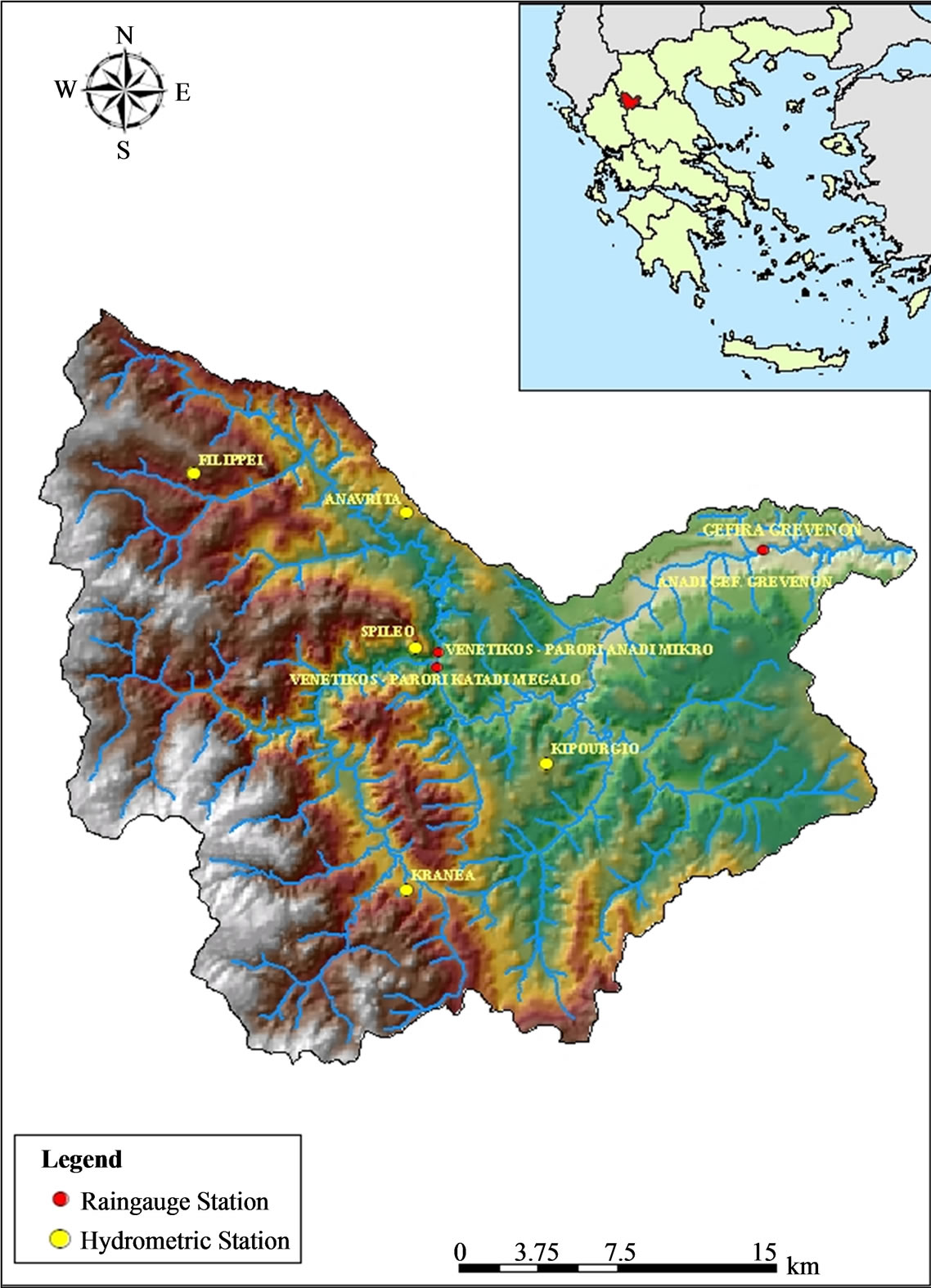
Figure 1. The study area.

Table 1. General characteristics of the study area.
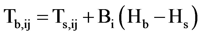
included precipitation, snow, evaporation, wind velocity, relative humidity, sunshine duration and temperature values. Precipitation data from a number of raingauge recording stations was used. Monthly areal precipitation was calculated by using the well-known Thiessen polygon method and corrected on the basis of a precipitation-elevation relationship. Temperature monthly values were obtained for each station and an average lapse rate Bi of monthly temperatures was estimated over the period of operation and for each month by associating the mean monthly temperature of each station with its elevation. A relation was established between the mean temperature of the stations of the basin Ts,ij (˚C) and the mean temperature at the mean elevation of the basin Tb,ij (˚C), as follows:
 (1)
(1)
where i denotes months and j denotes years, and Hb, Hs (in meters) are the mean elevations of basin and stations, respectively. Values for the mean monthly air temperature of the basin Tb are used directly in the water balance model for dividing precipitation into rain and/or snow, as well as in the snow melting algorithm. The mean monthly evapotranspiration, which is a direct input to the water balance model, is computed from field data according to the Blaney-Griddle and the Penman methods.
3. Methodology
Climate change scenarios reflecting future global increases in greenhouse gas concentrations constructed for Europe (including Greece), at 0.5˚ latitude/longitude resolution by the Climatic Research Unit (CRU) of the University of East Anglia, England (Hadley Centre, 1995) were used in this study. The methodology adopted used the constructed by the CRU 1961-90 baseline climatologies for Europe, the results from the GCM climate change experiment (UKTR) and a range of proportions of global warming calculated by MAGICC (Model for the Assessment of Greenhouse gas Induced Climate Change), a simple up welling-diffusion energy balance climate model [13] .
The resulting climate change fields were applied to the baseline climatology presenting the 30-year period 1961-90. The fields include rainfall R (in % change), temperature T (in ˚C change) and potential evapotranspiration PE (in % change) [11] . Specifically, two scenarios were developed concerning the potential evapotranspiration, thus, PE1 representing change in potential evapotranspiration from a change in temperature only, and PE2 representing change in potential evapotranspiration from changes in radiation, humidity and windspeed. The transient experiment using the high resolution coupled ocean-atmosphere GCM of the Hadley Centre, UKTR, gave climate change scenarios for the decade 66 - 75 with a climate sensitivity of 2.5˚, assuming no sulphate aerosol effect corresponding to the year 2080.
Concisely, the process that was followed consists of the main steps given below:
• Application of the gridded historical data sets on transient climate scenario led to GCM output of the variables precipitation, temperature and evapotranspiration for the year 2080. The output grid resolution is 3.75˚ × 2.5˚ and the results are expressed in change of the above mentioned variables.
• Interpolation of the GCM output to 0.50 × 0.50 from the original GCM resolution (3.750 × 2.50 UKTR) and determination of a weighting coefficient for each cell.
• Estimation of the monthly surface value of precipitation, temperature and evapotranspiration of the year 2080 by multiplying the weighting coefficient of each cell with the respective value of change.
• Production of synthetic series (from 1990 up to 2080) of precipitation, temperature and potential evapotranspiration, which was based on the historical data (base run) and on the climate change scenario.
• Calibration of the water balance model. The Nash-Sutcliffe coefficient of efficiency was used as a criterion to monitor the accuracy of the calibration. The model outputs are the basin runoff and the soil moisture.
The results based on transient scenario were extracted from the gridded historical global data sets that include variables such as precipitation, temperature, windspeed, sunshine hours, vapour pressure and rain day frequencies, which were acquired by and processed at the Climatic Research Unit. The GCM output of the variables precipitation, temperature and evapotranspiration was interpolated to 0.5˚ × 0.5˚ from the original GCM resolution (3.75˚ × 2.5˚ UKTR) for the application of the climate change scenarios. The cell of 3.75˚ × 2.5˚ was divided into five cells of 0.5˚ × 0.5˚ towards the 2.5˚ dimension and to seven cells towards the 3.75˚ dimension. The rest 0.25˚ of the initial 3.75˚ cell was assigned the value of the sum of the two adjusted 3.75˚ × 2.5˚ cells, divided by two. The precipitation, temperature and evapotranspiration values were estimated by using the provided original gridded data and through the appropriate use of a weighting coefficient associated with each grid constituting the basin. The code number of each cell is calculated based on the longitude and latitude of the south west corner of the cell through the use of the following relation: Code = ((longitude + 180.0) × 100000.0) + ((latitude + 90.0) × 10.0) [13] .
It should be mentioned that the obligations of Greece under the UNFCC Convention are being fulfilled jointly with the other EU member states. For Greece, the agreed figure was a realistic objective to restrict the overall increase of CO2 up to +15% ± 3% by 2000 compared to 1990 levels, which was achieved based on the proposed initiated scenario. The ‘Burden Sharing Agreement’, which was finalized during the Environment Council of the EU in June 1998, proposes that Greece reduces the emissions of the six GH gases for the period 2008-2012 by +25% compared to the 1990 levels [14] . It was also decided to reduce emissions of the six gases to the atmosphere in 2020 by 20%. This shall be achieved by the implementation of a National Programme (http://www.minenv.gr/4/41/e4100.html), whose progress of implementation must be reported annually to the European Union Monitoring Mechanism. To achieve harmonization of the reported data and enable direct comparisons across sectors and between different countries all emission estimates should be reported following the methodology suggested by the Revised 1996 IPCC Guidelines for National Greenhouse Gas Inventories [15] .
4. Water Balance Model
The water balance model was utilised for the assessment of the climate change effects on the surface runoff of the study region, as described in previous publications [16] -[18] . It is a physically based water balance model, which operates on a monthly time step.
The input parameters which were used for the calibration of the conceptual water balance model are the maximum soil moisture parameter, the watershed lag coefficient, the groundwater reservoir coefficient, the temperature parameters (lower T0 and upper T1 thresholds), the minimum rain content coefficient, the melt-rate factor and the storm runoff coefficient [19] .
More specifically, the maximum soil moisture is a basin average of the moisture holding capacity of upper soil zone. The watershed lag coefficient is the parameter applied on the water surplus in order to yield the amount of water that will eventually flow to the river course within a month, after having fulfilled the requirements of evapotranspiration and soil moisture replenishment, while the groundwater reservoir coefficient is the rate of outflow from the groundwater storage to the river course, considered to occur with a lag of one month. A simple snow melting subroutine based on temperature thresholds, minimum rain content coefficient and a melt-rate factor was applied for the calculation of the snow melt values. Particularly, the model estimates the rain and snow from the total precipitation according to monthly average basin temperature and to the temperature thresholds (T0 and T1). Below the temperature T0 the snow content of areal precipitation reaches a maximum, between T0 and T1 it is linearly dependent on temperature and above T1 precipitation falls entirely as rain [16] . The snow-tank, which is the amount of the accumulated snow at the end of each month, and the snow melt, which is the quantity of snow melting each month, are calculated through the use of the snow melting subroutine. However, it should be mentioned that due to the monthly time scale of the model (values of mean monthly temperatures are used), the produced values of snow are underestimated. A daily based model would have produced more realistic snow, snow-tank and snow melt values. Finally, the storm runoff coefficient determines how much of the water falling as rain flows directly as storm runoff before any other processes take place. This parameter depends on the month of the year therefore, twelve values were determined.
The final values of the input parameters were derived during the calibration phase of the model and were used in the application of the model with the climate change scenario. Outputs of the model are the basin runoff and the soil moisture values. The soil moisture is the quantity of water held in the aeration zone, which can supply water for evapotranspiration when the surface water does not suffice. The Nash coefficient was used as a criterion regarding the accuracy of the calibration. The calibration was performed twice, firstly by incorporating the Blaney-Criddle method and secondly by incorporating the Penman one, which was initially suggested to be applied, for the calculation of the potential evapotranspiration. Since the values of the Nash parameters obtained in the first case were higher than the values obtained in the second case, the Blaney-Criddle method was selected and used for the application of the model. Furthermore, runs of the water balance model were also conducted using the proposed by the CRU scenarios PE1 and PE2, regarding the potential evapotranspiration, as mentioned previously. It was found that the runoff values, which were estimated by using the scenarios PE1 and PE2 did not significantly differ from the ones, where the Blaney-Criddle method was applied simultaneously with the precipitation and temperature scenarios and therefore the Blaney-Criddle method was finally used for the application of the model.
5. Results
In order to apply the climate change scenarios to the hydrometeorological data, synthetic series (from 1990 up to 2080) of precipitation, temperature and potential evapotranspiration based on the historical data, were produced. Two stochastic autoregressive models AR(1) and AR(2) were applied to the historical data (30 year period) and the test Portmanteau was used as a the criterion to check their efficiency in each case. Finally, 50 synthetic series of each variable were generated in order to be used as inputs in the water balance model with or without the scenarios.
During the next phase of work, the constructed by the CRU 1961-90 baseline data (0.5˚ latitude/longitude resolution) of precipitation, temperature and potential evapotranspiration (12 mean monthly values) were compared to the mean monthly historical data in order to determine the reference base for scenario application. The mean historical data were used instead of the baseline data since the observed differences were not so significant. The climate change scenarios were finally applied to the hydrometeorological generated series by correcting each of their monthly value using a linear interpolation between the generated values and the corresponding mean monthly historical values.
For comparison reasons, Figure 2 presents the constructed by the CRU mean monthly values of precipitation, temperature and potential evapotranspiration for 1961-90, as well as the equivalent mean values of the historical observed climatological data. From this comparison, it occurred that the winter temperature was slightly underestimated, while potential evapotranspiration was overestimated. Therefore, it was decided that for accuracy reasons due to catchment scale, the mean historical data should be used instead of the baseline climatology since the observed differences were not so significant.

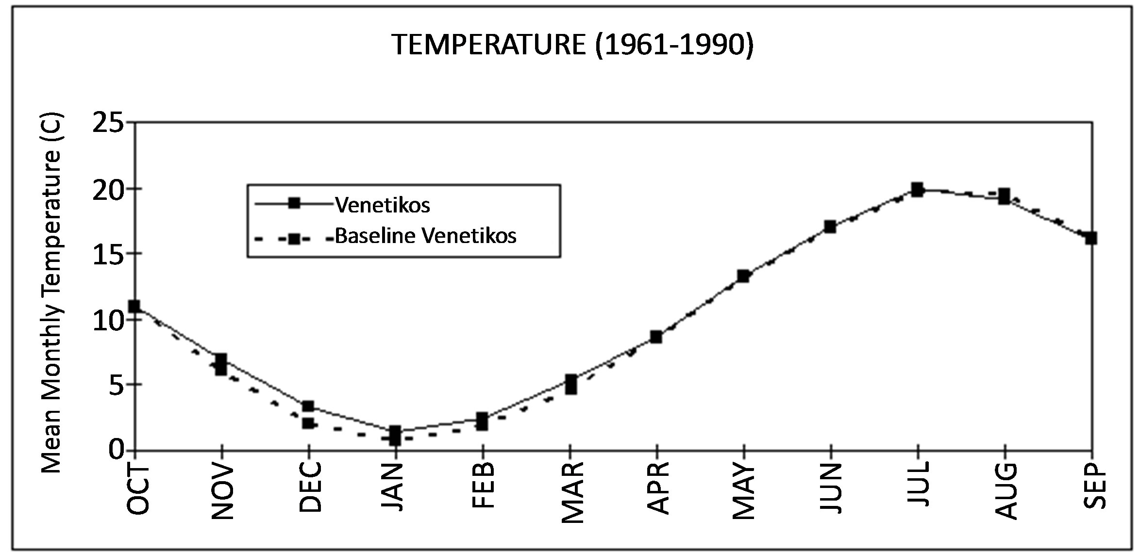
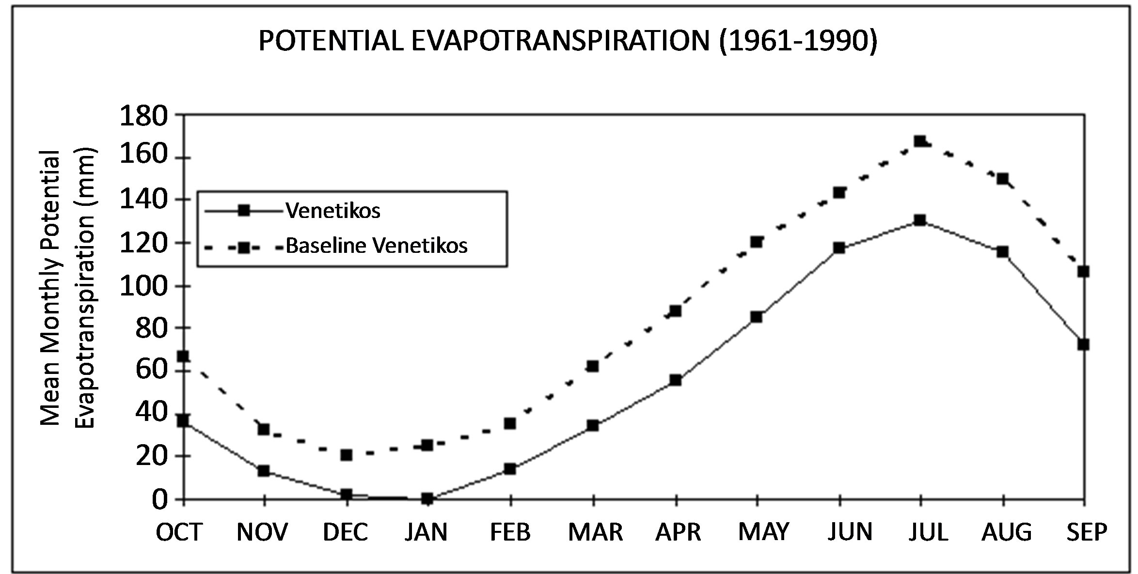
Figure 2. Comparison of the constructed by the CRU 1961-90 baseline climatology to the mean historical precipitation, temperature and potential evapotranspiration values.
The climate change scenarios were finally applied to the hydrometeorological generated series by correcting each of their monthly value using a linear interpolation between the generated values and the corresponding mean monthly historical values. Runs of the water balance model in order to estimate possible future runoffs for all time steps, using the already generated hydrometeorological data and considering zero climate change (no application of climate change scenarios), are referred to as base runs and were used for comparison purposes. The selection of the base runs as a basis of comparison was made for uniformity reasons and it was accepted since each base run was found to be similar to the historical record. Figures 3 and 4 depict the mean monthly runoff values and the mean monthly actual evapotranspiration, estimated by the PE1, PE2 and the Blaney-Criddle method. One can notice slight differences among the three cases, justifying thus the use of the Blaney-Criddle method for all base runs.
In order to make optimal use of all produced results, several hydrological indicators were selected and compared such as mean annual runoff, mean monthly runoff, mean annual maximum and minimum runoff values. From Table 2, referring to the abovementioned period 1990-2080, it is seen that reduction of the mean annual runoff values would occur in all cases, as well as serious reduction of summer runoff, while the wet period is shifted towards December resulting in prolongation of the dry period. The mean annual potential evapotranspiration
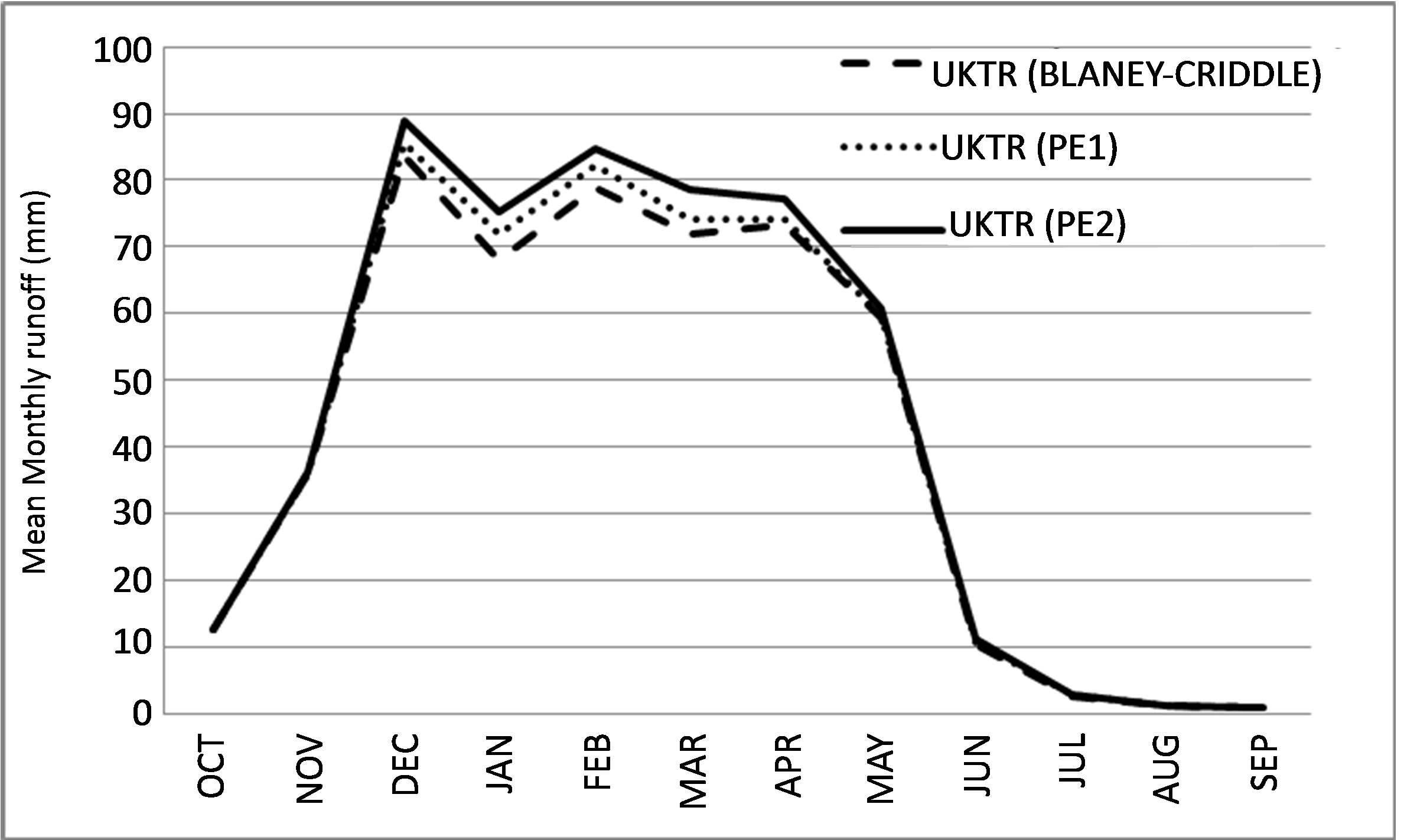
Figure 3. Mean monthly runoff of the basin estimated by applying the PE1, PE2 and the Blaney-Criddle method.
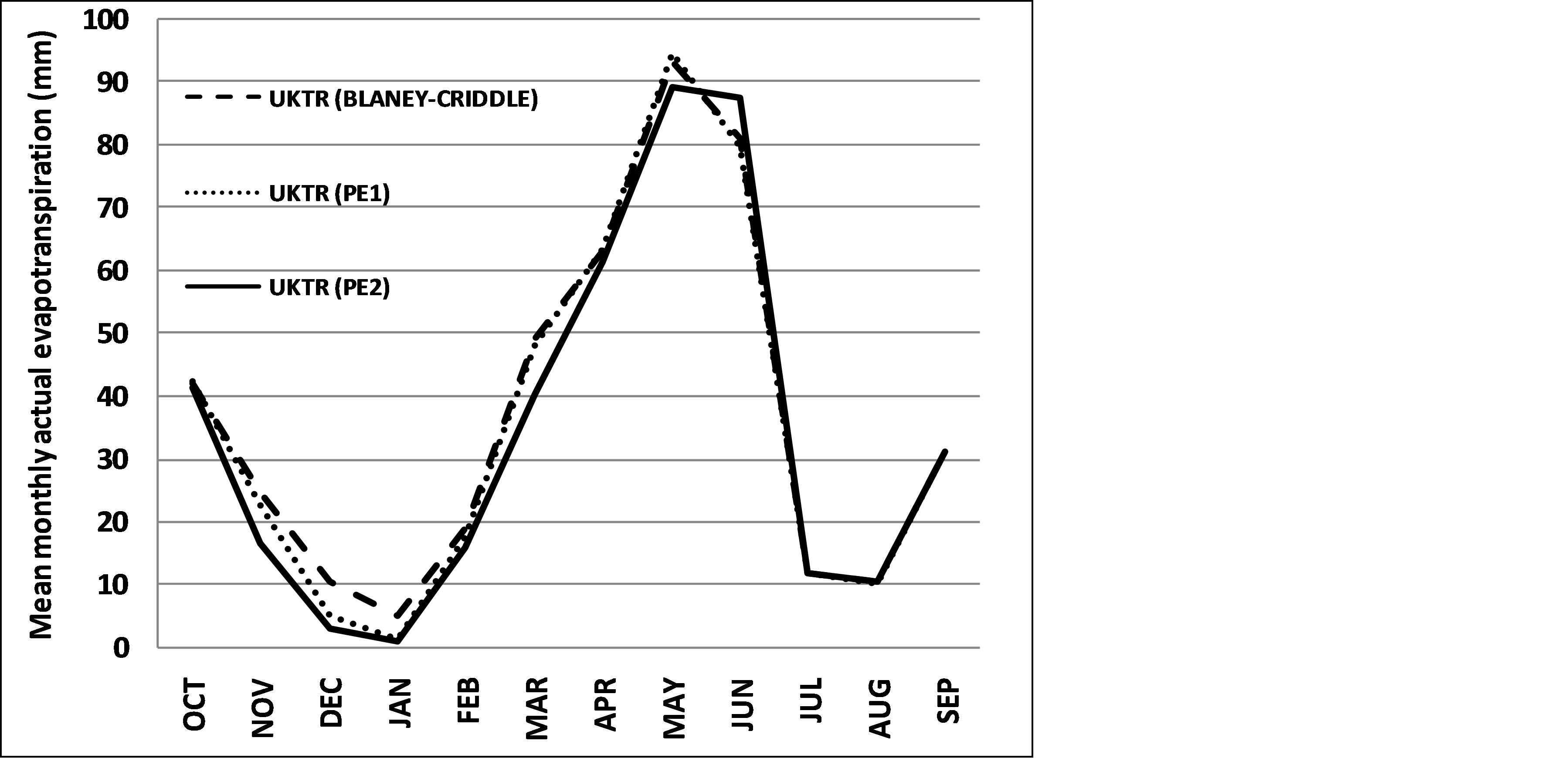
Figure 4. Mean monthly actual evapotranspiration of the basin estimated by applying the PE1, PE2 and the Blaney-Criddle method.
Table 2. Presentation of changes of hydrological indicators from the application of transient climate change scenario UKTR for the period 1990-2080.
values would eventually increase due to temperature increases.
Figure 5 shows the estimated mean monthly runoff values (mm) of the basin for the period 1990-2080, resulting from the above procedure. A reduction in the mean monthly runoff is observed, especially in the winter months. The mean actual evapotranspiration is shown in Figure 6, in which a substantial increase is observed all year except for the summer months. The temperature increase results in reduction of snow accumulation and decrease of spring runoff values and soil moisture. The annual runoff and the summer annual runoff are depicted in Figures 7 and 8. It was found that the mean annual runoff in the transient scenario will be reduced by 22% compared to the base run scenario, while the mean summer runoff by 13% respectively.
6. Conclusions
The basic conclusions drawn from this research are concentrated on the following:
• A monthly physically based water balance model was applied in a mountainous basin for the assessment of the climate change effects on the surface runoff of the study region.
• The Blaney-Criddle method was used, since its simultaneous application with the precipitation and temperature scenarios did not differ from the proposed by CRU scenarios PE1 and PE2.
• The mean annual, mean winter and mean summer runoff values were decreased compared to the base run scenario for 21.9%, 23.5% and 13% respectively, while the potential evapotranspiration was increased for 20.4%, resulting in a reduction of soil moisture.
• The wet period was shifted towards December resulting in severe prolongation of the dry period.
• Due to the monthly time scale of the model (values of mean monthly temperatures are used), the produced values of snow are underestimated. A daily based model would have produced more realistic snow, snowtank and snow melt values.
The impact of climate change on the hydrological regime and the water resources in the Venetikos basin should be taken seriously into consideration for the design of hydraulic projects in the area. A reduction of the
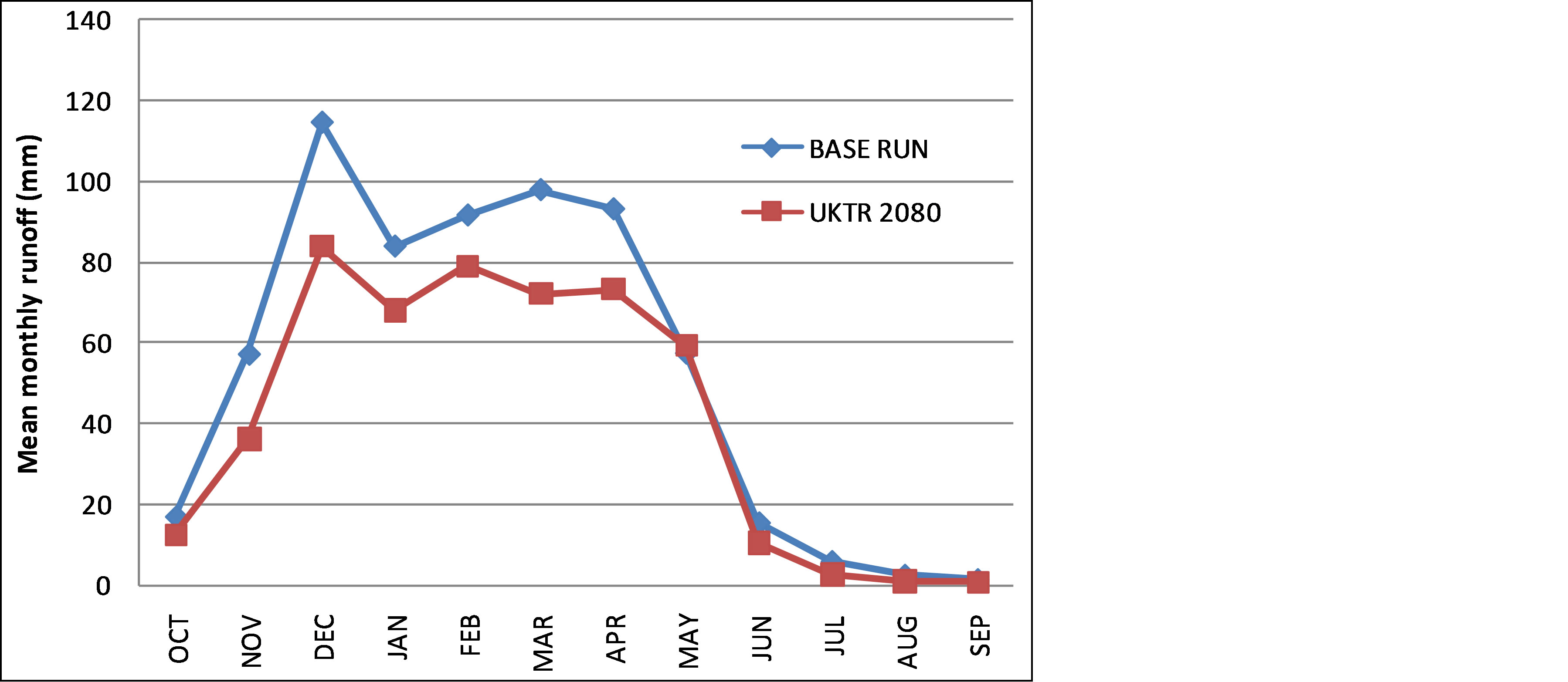
Figure 5. Mean monthly runoff of the Basin estimated by applying the transient scenario UKTR for the period 1990-2080.

Figure 6. Mean monthly actual evapotranspiration of the Basin estimated by applying the transient scenario UKTR for the period 1990-2080.
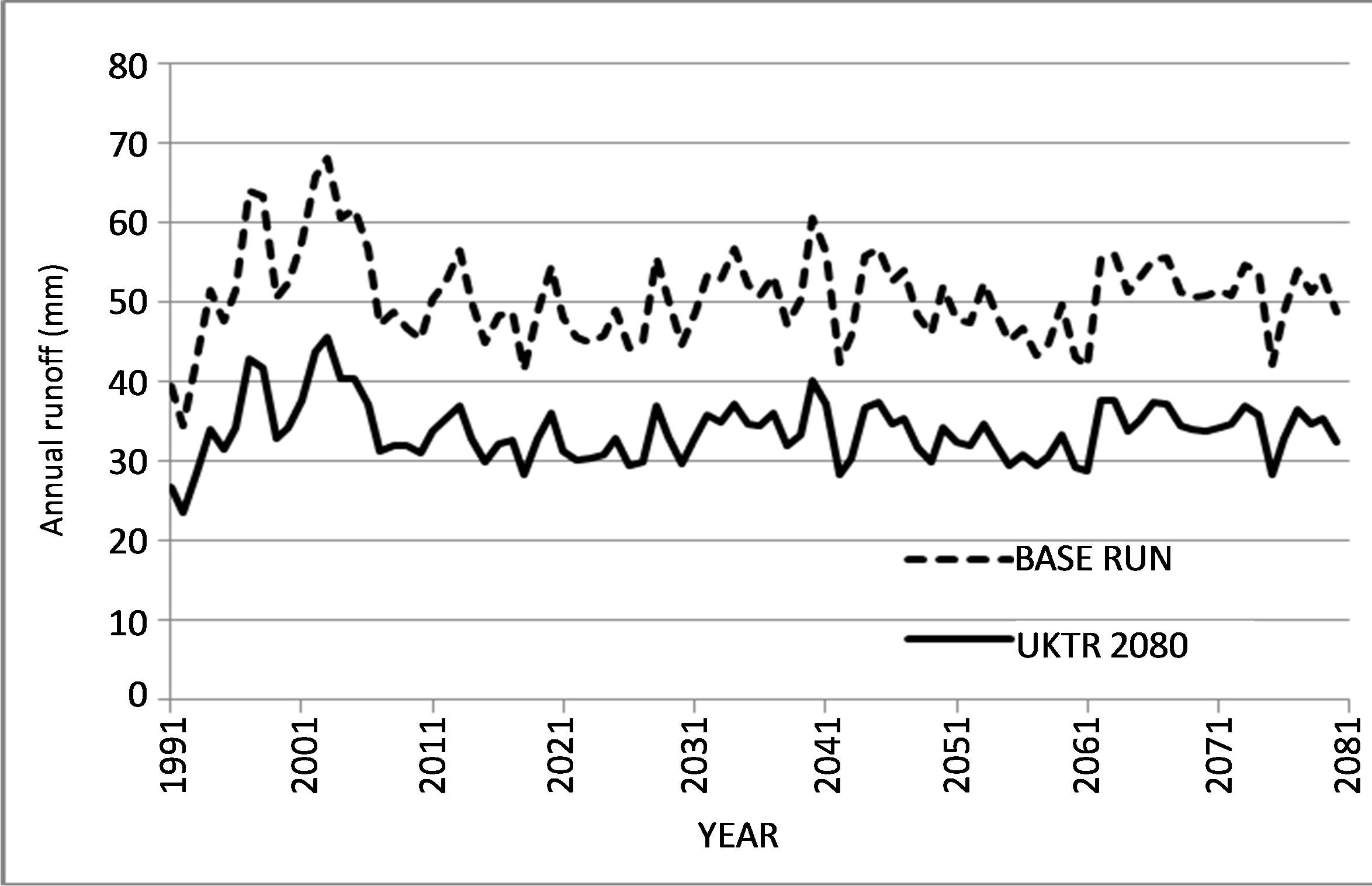
Figure 7. Annual runoff estimated by applying the transient scenario UKTR for the period 1990-2080.
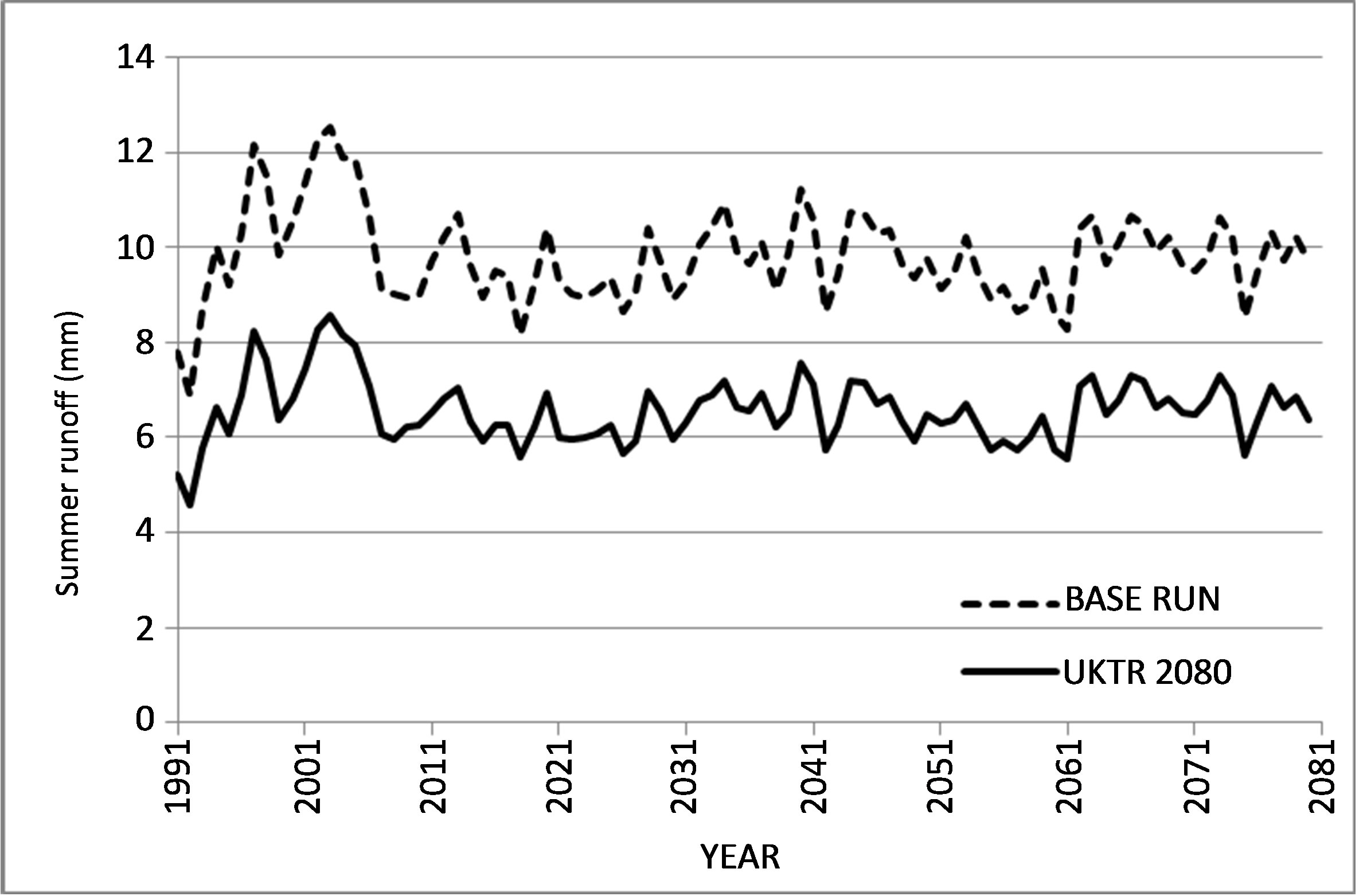
Figure 8. Summer annual runoff estimated by applying the transient scenario UKTR for the period 1990-2080.
mean annual runoff and the prolongation of the dry period could severely affect the regional economy, since it is mainly based on agriculture and pastoral farming.
References
- IPCC (2000) Third Assessment Report, Working Group I Report. Cambridge University Press, Cambridge.
- Arnell, N.W. (2004) Climate Change and Global Water Resources: SRES Emissions and Socio-Economic Scenarios. Global Environmental Change, 14, 31-52. http://dx.doi.org/10.1016/j.gloenvcha.2003.10.006
- Ashiq, M.W., Zhao, C., Ni, J. and Akhtar, M. (2009) GIS-Based High-Resolution Spatial Interpolation of Precipitation in Mountain-Plain Areas of Upper Pakistan for Regional Climate Change Impact Studies. Theoretical and Applied Climatology, 99, 239-253.
- Christensen, N.S., Wood, A.W., Voisin, N., Lettenmaier, D.P. and Palmer, R.N. (2004) The Effects of Climate Change on the Hydrology and Water Resources of the Colorado River Basin. Climatic Change, 62, 337-363.
- Evans, J. and Schreider, S. (2002) Hydrological Impacts of Climate Change on Inflows to Perth, Australia. Climatic Change, 55, 361-393. http://dx.doi.org/10.1023/A:1020588416541
- Hagemann, S., Gottel, H., Jacob, D., Lorenz, P. and Roeckner, E. (2009) Improved Regional Scale Processes Reflected in Projected Hydrological Changes over Large European Catchments. Climate Dynamics, 32, 767-781. http://dx.doi.org/10.1007/s00382-008-0403-9
- Kostopoulou, E., Giannakopoulos, C., Anagnostopoulou, C., Tolika, K., Maheras, P., Vafiadis, M. and Founda, D. (2007) Simulating Maximum and Minimum Temperature over Greece: A Comparison of Three Downscaling Techniques. Theoretical and Applied Climatology, 90, 65-82.
- Middelkoop, H., Daamen, K.. Gellens, D., Grabs, W., Kwadijk, J.C., Lang, H., Parmet, B.W., Schädler, B., Schulla, J. and Wilke, K. (2001) Impact of Climate Change on Hydrological Regimes and Water Resources Management in the Rhine Basin. Climatic Change, 49, 105-128. http://dx.doi.org/10.1023/A:1010784727448
- Vanrheenen, N., Wood, A., Palmer, R. and Lettenmaier, D. (2004) Potential Implications of PCM Climate Change Scenarios for Sacramento, San Joaquin River Basin. Climatic Change, 62, 257-281. http://dx.doi.org/10.1023/B:CLIM.0000013686.97342.55
- Vörösmarty, C.J., Green, P., Salisbury, J. and Lammers, R.B. (2000) Global Water Resources: Vulnerability from Climate Change and Population Growth. Science, 289, 284-288. http://dx.doi.org/10.1126/science.289.5477.284
- Mitchel, T. and Hulme, M. (2000) A Country by Country Analysis of Past and Future Warming Rates. Tyndall Centre Internal Report, 1 November 2000, UEA, Norwich, 6 p. http://www.tyndall.uea.ac.uk/main.htm
- Boorman, D.B. and Sefton, C.E.M. (1997) Recognising the Uncertainty in the Quantification of the Effects of Climate Change on Hydrological Response. Climatic Change, 35, 415-434.
- Hulme, M., Conway, D., Brown, O. and Barrow, E. (1994) A 1961-90 Baseline Climatology and Future Climate Change Scenarios for Great Britain and Europe. Climatic Research Unit, University of East Anglia.
- IPCC (1992) Climate Change 1992: The Supplementary Report to IPCC Scientific Assessment. Cambridge University Press, Cambridge.
- IPCC (1996) Climate Change 1995: The Science of Climate Change (Contribution of Working Group I to the Second Assessment Report of the Intergovernmental Panel on Climate Change). Cambridge University Press, Cambridge.
- Baltas, E. and Mimikou, M. (2005) Climate Change Impacts on the Water Supply of Thessaloniki. Journal of Water Resources Development, 21, 341-353. http://dx.doi.org/10.1080/07900620500036505
- Baltas, E.A. (2007) Impact of Climate Change on the Hydrological Regime and Water Resources in the Basin of Siatista. Journal of Water Resources Development, 23, 501-518. http://dx.doi.org/10.1080/07900620701485980
- Baltas, E.A. (2009) Climate Change and the Associated Implications on the Water Policy Framework in the Basin of Venetikos. Journal of Water Resoures Development, 25, 491-506. http://dx.doi.org/10.1080/07900620902972661
- Baltas, E.A. and Karaliolidou, M.C. (2010) Land Use and Climate Change Impact on the Reliability of Hydroelectric Energy Production. Journal of Strategic Planning for Energy and the Environment, 29, 56-73. http://dx.doi.org/10.1080/10485231009709883