Journal of Geoscience and Environment Protection
Vol.07 No.03(2019), Article ID:91478,13 pages
10.4236/gep.2019.73010
Spatial and Temporal Variations in Available Soil Nitrogen―A Case Study in Kobresia Alpine Meadow in the Qinghai-Tibetan Plateau, China
Li Lin1, Guangmin Cao1, Fawei Zhang2*, Xun Ke1, Yikang Li1, Xingliang Xu3, Qian Li1, Xiaowei Guo1, Bo Fan1, Yangong Du1
1Northwest Institute of Plateau Biology, Chinese Academy of Science, Xining, China
2College of Life Science, Luoyang Normal University, Luoyang, China
3Key Laboratory of Ecosystem Network Observation and Modeling, Institute of Geographic Sciences and Natural Resources Research, Chinese Academy of Sciences, Beijing, China

Copyright © 2019 by author(s) and Scientific Research Publishing Inc.
This work is licensed under the Creative Commons Attribution International License (CC BY 4.0).
http://creativecommons.org/licenses/by/4.0/


Received: January 10, 2019; Accepted: March 25, 2019; Published: March 28, 2019
ABSTRACT
Elucidating the factors that determine the effects of temporal and spatial variation of nutrients is important for analyzing the characteristics of an ecosystem. The goal of this paper was to estimate how values obtained using a particular sampling approach correlated with the actual data for an entire plot. The mesh partition method was employed to divide an integrated observing field (IOF) located at the Haibei National Field Research Station of an alpine grassland ecosystem, China, into 25 subplots. Five of the 25 subplots were randomly selected for soil sampling and to determine the source of variations in soil nutrient content from 2001 to 2012. The results showed that, contributions of temporal and spatial variation in available nitrogen in the 0 - 10 cm soil layer accounted for 47.3% and 52.7%, respectively. The contribution of spatial variance was higher than that of temporal variance especially in the surface soil layers. The available soil nitrogen content in the alpine meadow was not obviously affected by fluctuations in rainfall and temperature. Increasing the number of samples could reduce calculation errors in measuring available soil nitrogen content, while collecting a reasonable number of samples can save time and labor.
Keywords:
Available Soil Nitrogen, Source of Nutrient Variation, Temporal Variation, Spatial Variation, Alpine Meadow

1. Introduction
Soil nutrients are the dominant factor related to the productivity of natural ecosystems, affecting the dynamics of species and community composition, as well as the competition between individual species and within the plant community for limited soil nutrients (Ren et al., 2013) . Soil nutrient status often restricts the process of plant community succession and ecosystem responses to environmental change (Jing et al., 2014; Tian et al., 2019) . For most grassland ecosystems, nitrogen is one of the important factors limiting grassland productivity (Wei et al., 2013; Urakawa et al., 2016; Richard et al., 2019) . Grasslands are known to be sensitive to soil nitrogen enrichment (Bai et al., 2008; Yang et al., 2011) . Competition for soil nitrogen is considered as an important factor in determining the plant community secondary succession, especially in Qing-Tibetan Plateau (Niu et al., 2006; Dai et al., 2009; Lin et al., 2013) .
Although an abundant supply of atmospheric nitrogen and the soil organic nitrogen is available, to the vast majority of plants in an ecosystem is limited by the plant’s ability to absorb different forms of nitrogen (Liu et al., 2016) . Available nitrogen mainly refers to the sum of nitrate nitrogen and ammonium nitrogen in an ecosystem, the forms of nitrogen that plants can readily adsorb. Available nitrogen content has a certain temporal and spatial heterogeneity (Wang et al., 2014) . Spatial factors that cause variations in available soil nitrogen include precipitation, temperature, topography, rock mineralogical characteristics, soil texture, soil structure, soil fauna, microbial functional groups, plant community characteristics, types of litter, and root uptake and turnover (Tilman, 1987; Goovaerts, 1999; Rajaniemi, 2003; Du, 2009; Duprè et al., 2010; Kazuki et al., 2019) . Meanwhile, temporal factors that cause variations in available soil nitrogen include animal grazing and trampling intensities, deposition of excreta, fires and other external factors and ecosystem management measures (Dalva & Moore, 1991; van Wijnen et al., 1999 ; Gao et al., 2004; Flessa et al., 2000; Uselman et al., 2000) . The effect of spatial heterogeneity, in essence, involves hydrothermal redistribution, and hydrothermal heterogeneity causes the heterogeneity in community development and composition and in soil nutrients (Lozano et al., 2014) . The effects of temporal heterogeneity in non-cultivated grassland, in essence, include climate and disturbance, such as different stocking levels or animal grazing. In addition, the grazing of livestock affects grassland through the ingestion of plants and plant trampling. Long-term grazing exclusion significantly affected the heterogeneity, dominant species and community composition of alpine grasslands (Jing et al., 2014) . This change is unpredictable. Grazing could increase the spatial heterogeneity of soil nutrients through the deposition of manure. However, grazing could also reduce the effects of spatial heterogeneity by the ingestion of plants by animals (Lozano et al., 2014) .
Elucidating the factors that determine the effects of temporal and spatial variation in available soil nitrogen presents a major challenge during an analysis of ecosystem characteristics. Determining such variations arising from a temporal or spatial scale is essential. Geostatistics as well as statistical theories and methods are often used to analyze the spatial variability of soil nutrients. However, using geostatistics requires an adequate number of samples and an appropriate sampling scale (Zhu et al., 1997) , so it is not suitable for the analysis temporal and spatial heterogeneity at any one point in time and scale. Multivariate analysis (MVA), one of the approaches of the study of random-effects of nested statistical analysis, is widely used to assess the source of variation in an experiment (Montgomery, 1997) . MVA is used to assessing the variation in experimental data based on a linear statistical hypothesis. The hypothesis of MVA is that variation effects in statistical data are independent of each other, and all the statistical data have no interactive effects between each other (Douglas, 2004; Peng, 2010) . This approach might explain the variation in parameters in experiments in order to identify ways to deal with the sources of variation, and elucidate methods that can be used to rectify spatial or temporal variation.
Alpine grasslands serve as one of the most important grassland types on earth, and are distributed across the tundra zone of northern Eurasia and
In this study, we used 12 years of available soil nitrogen data from the Haibei National Field Research Station and the alpine grassland ecosystem in Qinghai, China. Our aim is to determine the extent of the contribution of temporal and spatial factors to variations in soil nutrients, using multivariate analysis (MVA).
2. Materials and Methods
2.1. Sampling Design, Field Investigation, and Laboratory Analyses
The study area is located in the Haibei National Field Research Station of Alpine Grassland Ecosystem of the Qinghai-Tibetan Plateau (37˚29'N, 101˚12'E, 3200 m), Chinese Academy of Sciences, Qinghai, China (HGB). The average annual precipitation and temperature were 582.1 mm and −1.7˚C, respectively. The warmest and coldest months, were July and January, respectively. The dominant plants in the community were Stipa spp., Festuca spp., and Kobresia humilis in the integrated observing field (IOF) of this research station, an area with a high degree of plant community evenness. The growing season was from May to September, while plant community biomass peaked in August.
Grazing intensity in the study area was 2.01 sheep unit per hectare. The IOF had no fertilizer applied in the study area. Livestock grazed in the IOF from November to the end to May of the next year from 2001 to 2007, but only from November to the end of March of next year from 2008 to 2012. We divided the IOF (100 m × 100 m) into 25 subplots (20 m × 20 m) and sampled soils using five earth-auger borings (Ф = 6 cm) within each subplot. Three sets of soil layers were sampled: samples from depths of 0 - 10 cm, 10 - 20 cm and a combined sample of 0 - 20 cm, at the end of August in every year during 2001 to 2012. In each year, we randomly selected 5 - 25 subplots in the diagonal in the IOF to analyze the spatial variance in soil conditions. In addition, in 25 selected subplots, the 0 - 20 cm soil layers were used to analyze what would happen when increasing the sampling number from 5 to 25. Available soil nitrogen content was considered as nitrogen in the form of total ammonium-nitrogen and nitrate-nitrogen. The data for ammonium- and nitrate-nitrogen content were obtained using a flow analyzer (Skala, Holland) by using 2-mm grain size fresh soil.
The data of total nitrogen and soil organic matter content from the 0 - 10 cm and 10 - 20 cm soil samples were obtained using elemental analyser (PE2400II, America) by using 0.25-mm grain size air-dried soil.
The data of the accumulated rainfall and temperature data were obtained from the Haibei National Field Research Station of Alpine Grassland Ecosystem weather station (37˚29'N, 101˚12'E, 3200 m) from 2001 to 2012.
2.2. Statistical Analysis
All statistical analyses were completed and all graphs were produced using the SPSS19.0 software package for Windows and Excel 2003.
MVA was based on a linear statistical model as seen in Equation (1):
, (1)
where u is the average without considering the variations in temporal and spatial factors, ti represents the effects of temporal variation in different years, and β(i)j represents the spatial variation in different subplots. The spatial and temporal variances were determined as Equation (2):
, (2)
where σTotal is the total temporal and spatial variance, and σт is temporal variation, and σβ is the spatial variation.
Let , and .
The total sum of squared deviations is provided in Equation (3):
(3)
Then, Equation (4) shows:
, (4)
where SS denotes the sum of squared deviations, MS is the standard error, and n is the degrees of freedom. Therefore, the variation in variance estimation was determined as described by Dean and Voss (1999) and Peng (2010) as Equations (5) and (6):
, (5)
(6)
The variations of the available soil nitrogen content between soil layers and sampling subplots and years were estimated using one-way analysis of variance.
The data range is shown in Equation (7):
, (7)
where dr represents the data range, xmaxi represents the largest soil nitrogen content in the group, and xmin represents the smallest soil nitrogen content in the group.
Arithmetic mean deviation was calculated using Equation (8):
, (8)
where amd represents the arithmetic mean deviation, represents arithmetic mean, and xi represents the observed soil nitrogen content.
3. Results
3.1. Temporal Heterogeneity in the IOF
Available soil nitrogen content fluctuated inter-annually in the 0 - 10 cm soil layer with the mean nitrogen content of 21.8 ± 1.4 mg・kg−1 (coefficient of variation, 6.4%) during the 12 years of the study period (Figure 1). In the first 7 years, the available soil nitrogen fluctuated remarkably in the IOF with a mean content of 22.2 ± 6.2 mg・kg−1 (coefficient of variation, 27.4%). However, from 2008 to 2012, grazing livestock was prohibited in the growing seasons in the IOF, and the available soil nitrogen content fluctuated more consistently and steadily,
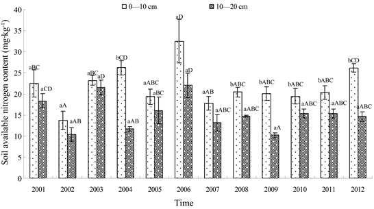
Figure 1. The soil available nitrogen contents during 2001 to 2012 in different soil layers. Note: the capital letters are on behalf of significant coefficient between different years, the lowercase letters are on behalf of the significant coefficient between different soil layers.
with a mean content of 21.3 ± 2.8 mg・kg−1 (coefficient of variation, 13.0%; Figure 1); this value was considerably lower than that in the first 7 years.
Available soil nitrogen content in the 10 - 20 cm soil layer also fluctuated inter-annually, but the values were lower than that in the 0 - 10 cm soil layer (Figure 1). The mean nitrogen content was 15.2 ± 3.9 mg・kg−1 (coefficient of variation, 25.3%) during the 12 years of the study period. In the first 7 years, the available soil nitrogen content fluctuated remarkably in the IOF, in that the mean available soil nitrogen was 16.2 ± 4.7 mg・kg−1 (coefficient of variation, 28.9%). However, from 2008 to 2012, the mean available soil nitrogen was 13.9 ± 2.1 mg・kg−1 (coefficient of variation, 15.1%; Figure 1).
In the first 7 years, the available soil nitrogen content was not significantly different between the 0 - 10 cm and 10 - 20 cm soil layers with the exception of 2004. Meanwhile, the available soil nitrogen content was significantly higher in 0 - 10 cm than in 10 - 20 cm soil layer during 2008 to 2012. The available soil nitrogen content did not vary significantly during 2001 to 2007 (α = 0.05). However, from 2008 to 2012 the available nitrogen varied significantly between the 0 - 10 cm and 10 - 20 cm soil layers (Figure 1).
3.2. Spatial Heterogeneity in the IOF
Increasing the number of samples decreased the coefficient of variation in the available nitrogen content in the 0 - 20 cm soil layer in the IOF with a coefficient of variation of 13.0%. However, if the sample number was increased to 25 in the five samples from those same subplots, the coefficient of variation decreased by 140.7%, while variation of the mean was decreased by 3.5% compared to the 5-plot sampling in 2001 (Table 1).

Table 1. The variability in 0 - 20 cm soil partitioning in the integrated observing field.
The mean nitrogen content was 18.4 ± 4.3 mg・kg−1 (coefficient of variation, 23.5%) during the entire 12 years of the study period (Figure 2), and the range of available nitrogen content during 2001 to 2012 was 16.9 mg・kg−1. To determine the distribution of the data, we divided the data into five groups, because when the number of samples is lower than 50, the number of groups should be no more than five (Ma, 1982) . The arithmetic mean deviation was 3.0 mg・kg−1 in the 0 - 20 cm soil layer during those years, and the range of available nitrogen divided by the arithmetic mean deviation was about 4.0 mg・kg−1, which was used for the class interval (Figure 2). The frequency distribution of available soil nitrogen contents was normal with 50% of the data distributed in the median area with the probability of data in the first and last groups being less than 17%.
3.3. Contribution of Temporal and Spatial Variance in the Available Nitrogen Content in the Soil
We divided the IOF into 25 units, and selected five of them, using MVA to separate the variation of spatial and temporal factors from the total variance in the 0 - 10 cm soil layer from 2001 to 2012. The results showed that temporal and spatial factors accounted for 47.3% and 52.7%, respectively, of the total variation of available soil nitrogen in the 0 - 10 cm soil layer. The contribution of spatial variance was higher than that of temporal variance (Table 2).
However, for the 10 - 20 cm soil layer of the five subplots in the IOF, 78.2% of the variance was caused by the temporal components, while 21.8% was caused by spatial factors. The contribution of temporal variance was higher than that of spatial variance (Table 2).
3.4. The Relationship between Available Soil Nitrogen and Environmental Factors
In all, four environmental factors were selected, i.e., soil total nitrogen, soil organic matter, accumulated temperature (in the growing season), and rainfall (in

Figure 2. The distribution characteristics of available nitrogen content in the plot.
Table 2. Contributions of temporal and spatial variation in available nitrogen in the 0 - 10 cm and 10 - 20 cm soil layers.
Note: MS, standard error.
the growing season), that might have some effects on the variability of available soil nitrogen in the 0 - 10 cm soil layer. Of the four factors, only soil organic matter had a significant linear correlation with available soil nitrogen (α = 0.05; Table 3).
The correlations between these four environmental factors with the nitrogen content in the 10 - 20 cm soil layer were also been investigated. None of the factors had a significant linear correlation with available soil nitrogen content (α = 0.05; Table 3).
4. Discussion
4.1. The Causes of Variability in Available Soil Nutrients
Both temporal and spatial factors can affect the availability of soil nutrients in the meadow. The available soil nutrients content in grassland showed higher spatial heterogeneity than in cultivated fields because of various climatic, physical, chemical, biological, soil matrix, topography, and other soil-forming factors (Dai et al., 2009, Gao et al., 2004, Jing et al., 2014, Liu et al., 2016) . Furthermore, grassland management coupled with modern human activities has been changing the spatial heterogeneity of soil nutrients. Therefore, estimating only the temporal heterogeneity of soil nutrients is becoming increasingly difficult, and the effects of both spatial and temporal factors on available soil nitrogen content need to be distinguished.
The degree of spatial variability of nutrient content in non-cultivated soil mostly depends on the nutrient source and the mobility of the soil and this causes soil nutrients to have a strong spatial autocorrelation (Li et al., 2012) . Soil organic matter, a nutrient material, is considered as the major source of soil nitrogen. Soil organic matter can serve as a soil nitrogen index because soil nitrogen accumulates as the soil formed and the soil nutrients stored. Therefore, in our study, the level of nutrients stored in the soil had some positive effects on
Table 3. The relationship between accumulated temperature, rainfall, soil organic matter, and total nitrogen in the 0 - 10 cm and 10 - 20 cm soil layers.
*Denotes a significant difference between the two analysis factors.
available nitrogen.
The soil matrix is considered to have low spatial heterogeneity in a fixed small-scale environment. However, available nitrogen is fluid and as a result had little significant correlation with rainfall and accumulated temperature during the 12 years of the present study. Therefore, we assumed that available nitrogen content was not changed by environmental factors such as rainfall, accumulated temperature and the matrix of the soil. During the sampling process, we collected all samples using the same degree of slope as well as the same slope and slope position in order to avoid the micro-environmental influences. Therefore, the spatial and temporal heterogeneity observed in the present study did not come from the effects of terrain.
Thus, the available soil nitrogen content is very stable in the natural meadow in this region.
Abiotic factors play important roles in community distribution in the landscape, but species interactions are more important within communities (Maria, 2004) . For example, engineer species affect plant community and environmental interactions and become “ecosystem engineer species” (Jones et al., 1994, 1997) . These species are able to create, maintain, or eliminate the habitat of other species by modulating environmental factors. Various plant and animal species have been shown to affect community attributes through their engineering activities (Flecker, 1996; Crooks & Khim, 1999; Wright et al., 2002; Perelman et al., 2003; Castilla et al., 2004; Fritz et al., 2004; Zhang et al., 2004) . Ecosystem engineer species create habitat patches where environmental conditions and resource availability differ substantially from the surrounding unmodified environment (Jones et al., 1994, 1997) . Alpine meadows have high species richness. When the stocking of animal grazing was prohibited in the growing season, several non-dominant species that were always suppressed by stocking grazing or trampling increased in abundance and played the roles of ecosystem engineer species in our research plot. These species could interact with their surrounding environment, changing the biological environment (Fritz et al., 2004) and available soil nutrients (Castilla et al., 2004) . This may be the reason that there was higher spatial heterogeneity than temporal heterogeneity in the available soil nitrogen at our sampling site. It is also not clear why a contrasting finding was obtained in the 10 - 20 cm soil layer. Further studies will be warranted to address this issue.
4.2. Reason for Selecting the Number of Samples Based on Temporal and Spatial Variability in a Plot
The IOF had 25 subplots with 5 - 6 samples mixed to obtain a single sample in each subplot. This led to a coefficient of variation of 5.4% based on this kind of sampling method in the IOF. While the samples were obtained from five subplots based on the sampling method described above to determine the available soil nitrogen content in the entire IOF, the coefficient of variation was 13.0% in 2001. Therefore, increasing the number of samples could decrease the coefficient of variation for the statistical data.
If we used the mean based on 25 subplots to estimate available soil nitrogen content in the entire IOF, that mean was 20.0 mg・kg−1, which was in the range of 13 - 24 mg・kg−1. If we used this range as the actual data of the IOF, and we used the mean derived from five subplots to estimate the available soil nitrogen content in the entire IOF, only 17% of the time (2 years out of 12 years) the mean value of available nitrogen of the entire experimental area was outside this range. It may have been random chance that created the values that were not precisely in the range of 13.0 mg・kg−1 to 24.0 mg・kg−1. This means that increasing the amount of data available can improve the accuracy of the data. However, if we use five samples in this field, we only bear less than 17% risk of encountering the extreme value. Therefore, we believe it is reasonable to select five samples in a plot with uniform soil texture covering an area of less than 100 m × 100 m.
5. Conclusion
The soil nutrient content is known to be affected by complex interactions of spatial and temporal factors in the field, and the stored soil nutrients had an effect more or less on available nitrogen.
Over a relatively short time period (for example, 12 years), the spatial variability of soil nutrients was found to play a more important role than the temporal variability of available soil nutrients.
Therefore, we assumed that available soil nitrogen in the alpine meadow would remain relatively constant, and a certain amount of variation in rainfall and accumulated temperature would not affect the soil nitrogen content during the 12 years.
If the number of samples taken in the field was increased, the mean soil nitrogen content of those would be approximately the same as the actual value. However, if fewer samples are used, the data might yield erroneous results. If we use only five samples in a 100 m × 100 m plot, we create a less than 17% risk of encountering an extreme value, so we believe it is reasonable to select five samples in a cultivated soil texture plot with an area of less than 100 m × 100 m.
Acknowledgements
This study was supported by the National Natural Science Foundation of China (Grant No. 31500368, Grant No. 41730752), Instrument function development technology innovation project of Chinese Academy of Sciences (Grant No. 2020g106).
Conflicts of Interest
The authors declare that they have no conflict of interest.
Cite this paper
Lin, L., Cao, G. M., Zhang, F. W., Ke, X., Li, Y. K., Xu, X. L., Li, Q., Guo, X. W., Fan, B. & Du, Y. G. (2019). Spatial and Temporal Variations in Available Soil Nitrogen―A Case Study in Kobresia Alpine Meadow in the Qinghai-Tibetan Plateau, China. Journal of Geoscience and Environment Protection, 7, 177-189. https://doi.org/10.4236/gep.2019.73010
References
- 1. Bai, Y. F., Wu, J. G., Xing, Q. et al. (2008). Primary Production and Rain Use Efficiency across a Precipitation Gradient on the Mongolia Plateau. Ecology, 89, 2140-2153. https://doi.org/10.1890/07-0992.1 [Paper reference 1]
- 2. Castilla, J. C., Lagos, N. A., & Cerda, M. (2004). Marine Ecosystem Engineering by the Alien Ascidian Pyura praeputialis on a Mid-Intertidal Rocky Shore. Marine Ecology Progress Series, 268, 119-130. https://doi.org/10.3354/meps268119 [Paper reference 2]
- 3. Chen, D. R. (1982). A Preliminary Study of the Effect on N Fertilizer on Herbage Production and Nutrient Composition of Bromus inermis. Chinese Journal of Grassland, 4, 1–9. (In Chinese, English Summary) [Paper reference 1]
- 4. Crooks, J. A., & Khim, H. S. (1999). Architectural vs. Biological Effects of a Habitat-Altering, Exotic Mussel, Musculista senhousia. Journal of Experimental Marine Biology and Ecology, 240, 53-75. https://doi.org/10.1016/S0022-0981(99)00041-6 [Paper reference 1]
- 5. Dai, W., Zhang, R., Zhang, B., Du, Y. G. et al. (2009). Soil Fertility and Species Identity Control community Productivity in an Experimental Plant Community in an Area of Sub-Alpine Meadow—China. Chinese Journal of Plant Ecology, 33, 45-52. (In Chinese, English Summary) [Paper reference 3]
- 6. Dean, A., & Voss, D. (1999). Design and Analysis of Experiments (pp. 649-657). New York: Springer-Verlag. [Paper reference 1]
- 7. Dalva, M., & Moore, T. R. (1991). Sources and Sinks of Dissolved Organic Carbon in a Forested Swamp Catchments. Biogeochem, 15, 1-19. https://doi.org/10.1007/BF00002806 [Paper reference 1]
- 8. Douglas, C. M. (2004). Design and Analysis of Experiments (pp. 649-657). New Jersey: Wiley Press. [Paper reference 1]
- 9. Du, L. Y. (2009). The Study on the Soil Nutrients Special Heterogeneity of Different Forest in Changbai Mountain Area (pp. 2-4). Changchun: Northeast Normal University. [Paper reference 1]
- 10. Duprè, C., Stevens, C. J., Ranke, T. et al. (2010). Changes in Species Richness and Composition in European Acidic Grasslands over the Past 70 Years: The Contribution of Cumulative Atmospheric Nitrogen Deposition. Global Change Biology, 16, 344-357. https://doi.org/10.1111/j.1365-2486.2009.01982.x [Paper reference 1]
- 11. Flecker, A. S. (1996). Ecosystem Engineering by a Dominant Detritivore in a Diverse Tropical Stream. Ecology, 77, 1845-1854. https://doi.org/10.2307/2265788 [Paper reference 1]
- 12. Flessa, H., Ludwig, B., Heil, B. et al. (2000). The Origin of Soil Organic C, Dissolved Organic C and Respiration in a Long-Term Experiment in Halle, Germany, Determined by 13C Natural Abundance. Journal of Plant Nutrition and Soil Science, 163, 157-163. https://doi.org/10.1002/(SICI)1522-2624(200004)163:2<157::AID-JPLN157>3.0.CO;2-9 [Paper reference 1]
- 13. Fritz, K. M., Gangloff, M. M., & Feminella, J. W. (2004). Habitat Modification by the Stream Macrophyte Justicia American and Its Effects on Biota. Oecologia, 140, 388-397. https://doi.org/10.1007/s00442-004-1594-3 [Paper reference 2]
- 14. Gao, Y., Wang, S., Han, X. et al. (2004). Soil Nitrogen Regime and the Relationship between Aboveground Green Phytobiomass and Soil Nitrogen Fractions at Different Stocking Stocking Rates in the Xilin River Basin, Inner Mongolia. Acta Phytoecology Sinica, 28, 285-293. (In Chinese) https://doi.org/10.17521/cjpe.2004.0042 [Paper reference 2]
- 15. Goovaerts, P. (1999). Geostatistic in Soil Science: State-of-the-Art and Perspectives. Geoderma, 89, 1-45. https://doi.org/10.1016/S0016-7061(98)00078-0 [Paper reference 1]
- 16. Jing, Z. B., Cheng, J. M., Su, J. S. H. et al. (2014). Changes in Plant Community Composition and Soil Properties under 3-Decade Grazing Exclusion in Semiarid Grassland. Ecological Engineering, 64, 171-178. https://doi.org/10.1016/j.ecoleng.2013.12.023 [Paper reference 3]
- 17. Jones, C. G., Lawton, J. H., & Shachak, M. (1994). Organisms as Ecosystem Engineers. Oikos, 69, 373-386. https://doi.org/10.2307/3545850 [Paper reference 2]
- 18. Jones, C. G., Lawton, J. H., & Shachak, M. (1997). Positive and Negative Effects of Organisms as Physical Ecosystem Engineers. Ecology, 78, 1946-1957. https://doi.org/10.1890/0012-9658(1997)078[1946:PANEOO]2.0.CO;2
- 19. Kazuki, F., Miyabarab, Y., & Kunitoa, T. (2019). Microbial Biomass and Ecoenzymatic Stoichiometries Vary in Response to Nutrient Availability in an Arable Soil. European Journal of Soil Biology, 91, 1-8. https://doi.org/10.1016/j.ejsobi.2018.12.005 [Paper reference 1]
- 20. Li, X., Wanf, H., Yang, X. et al. (2012). A Review on Spatial Variability of Soil Nutrients Based on Geostatistics. Guangdong Agricultural Sciences, 22, 65-67, 76. (In Chinese) [Paper reference 1]
- 21. Lin, L., Li, Y. K., Zhang, F. W. et al. (2013). Soil Nitrogen and Phosphorus Stoichiometry in a Degradation Series of Kobresia humulis Meadows in the Tibetan Plateau. Acta Ecologica Sinica, 33, 5245-5251. (In Chinese) https://doi.org/10.5846/stxb201205310797 [Paper reference 1]
- 22. Liu, Y., He, N. P., Wen, X. F. et al. (2016). Patterns and Regulating Mechanisms of Soil Nitrogen Mineralization and Temperature Sensitivity in Chinese Terrestrial Ecosystems. Agriculture Ecosystems & Environment, 215, 40-46. [Paper reference 2]
- 23. Lozano, Y. M., Hortal, S., Armas, C. et al. (2014). Interactions among Soil, Plants, and Microorganisms Drive Secondary Succession in a Dry Environment. Soil Biology and Biochemistry, 78, 298-306. https://doi.org/10.1016/j.soilbio.2014.08.007 [Paper reference 2]
- 24. Ma, Y. H. (1982). Statistics for Experimenters (pp. 19-21). Beijing: Agricultural Press. [Paper reference 1]
- 25. Maria-Teresa, S. (2004). Role of Topography and Soils in Grassland Structuring at the Landscape and Community Scales. Basic and Applied Ecology, 5, 331-346. https://doi.org/10.1016/j.baae.2003.10.001 [Paper reference 1]
- 26. Montgomery, D. C. (1997). Design and Analysis of Experiments (4th ed., pp. 506-510). New York: John Wiley and Sons. [Paper reference 1]
- 27. Niu, K. C., Zhao, Z. G., Luo, Y. J. et al. (2006). Fertilization Effects on Species Reproductive Allocation in an Alpine Meadow Plant Community. Chinese Journal of Plant Ecology, 30, 817-826. (In Chinese) https://doi.org/10.17521/cjpe.2006.0104 [Paper reference 1]
- 28. Peng, X. (2010). Study on Multi-Vari Analysis of Statistic Process Control. Manufacturing Automation, 32, 140-143. [Paper reference 2]
- 29. Perelman, S. B., Burkart, S. E., & Leon, R. J. C. (2003). The Role of a Native Tussock Grass (Paspalum quadrifarium Lam.) in Structuring Plant Communities in the Flooding Pampa Grasslands, Argentina. Biodiversity & Conservation, 12, 225-238. https://doi.org/10.1023/A:1021948723714 [Paper reference 1]
- 30. Rajaniemi, T. K. (2003). Explaining Productivity Diversity Relationships in Plants. Oikos, 101, 449-457. https://doi.org/10.1034/j.1600-0706.2003.12128.x [Paper reference 1]
- 31. Ren, G. H., Deng, B., Shang, Z. H. et al. (2013). Plant Communities and Soil Variations along a Successional Gradient in an Alpine Wetland on the Qinghai-Tibetan Plateau. Ecological Engineering, 61, 110-116. https://doi.org/10.1016/j.ecoleng.2013.09.017 [Paper reference 1]
- 32. Richard, T., DeLaune, P. B., & Dowhower, S. L. (2019). Impacts of Over-Seeding Bermudagrass Pasture with Multispecies Cover Crops on Soil Water Availability, Microbiology, and Nutrient Status in North Texas. Agriculture, Ecosystems and Environment, 273, 117-129. https://doi.org/10.1016/j.agee.2018.12.013 [Paper reference 1]
- 33. Tian, L., Zhaoa, L., Wu, X. et al. (2019). Variations in Soil Nutrient Availability across Tibetan Grassland from the 1980s to 2010s. Geoderma, 338, 197-205. https://doi.org/10.1016/j.geoderma.2018.12.009 [Paper reference 1]
- 34. Tilman, D. (1987). Secondary Succession and the Pattern of Plant Dominance along Experimental Nitrogen Gradients. Ecological Monographs, 57, 189-214. https://doi.org/10.2307/2937080 [Paper reference 1]
- 35. Urakawa, R., Ohte, N., Shibata, H. et al. (2016). Factors Contributing to Soil Nitrogen Mineralization and Nitrification Rates of Forest Soils in the Japanese Archipelago. Forest Ecology and Management, 361, 382-396. https://doi.org/10.1016/j.foreco.2015.11.033 [Paper reference 1]
- 36. Uselman, S. M., Qualls, R. G., & Thomas, R. B. (2000). Effects of Increased Atmospheric CO2, Temperature, and Soil N Avail Ability on Root Exudation of Dissolved Organic Carbon by a N-Fixing Tree (Robinia pseudoacacia L.). Plant Soil, 222, 191-202. https://doi.org/10.1023/A:1004705416108 [Paper reference 1]
- 37. van Wijnen, H. J., van der Wal, R., & Bakker, J. P. (1999). The Impact of Herbivores on Nitrogen Mineralization Rate: Consequences for Salt Marsh Succession. Oecologia, 118, 225-231. https://doi.org/10.1007/s004420050722 [Paper reference 1]
- 38. Wang, C. T., Long, R. J., Wang, Q. L. et al. (2008). Response of Plant Diversity and Productivity to Soil Resources Changing under Grazing Disturbance on an Alpine Meadow. Acta Ecologica Sinica, 28, 4144-4152. [Paper reference 1]
- 39. Wang, W. J., Wang, H. M., & Zu, Y. G. (2014). Temporal Changes in SOM, N, P, K, and Their Stoichiometric Ratios during Reforestation in China and Interactions with Soil Depths: Importance of Deep-Layer Soil and Management Implications. Forest Ecology and Management, 325, 8-17. https://doi.org/10.1016/j.foreco.2014.03.023 [Paper reference 1]
- 40. Wei, L., Gang, Y., Huai, C. et al. (2013). Soil Available Nitrogen, Dissolved Organic Carbon and Microbial Biomass Content along Altitudinal Gradient of the Eastern Slope of Gongga Mountain. Acta Ecologica Sinica, 33, 266-271. https://doi.org/10.1016/j.chnaes.2013.07.006 [Paper reference 1]
- 41. Wright, J. P., Jones, C. G., & Flecker, A. S. (2002). An Ecosystem Engineer, the Beaver, Increases Species Richness at the Landscape Scale. Oecologia, 132, 96-101. https://doi.org/10.1007/s00442-002-0929-1 [Paper reference 1]
- 42. Yang, H. J., Li, Y., Wu, M. Y. et al. (2011). Plant Community Responses to Nitrogen Addition and Increased Precipitation: The Importance of Water Availability and Species Traits. Global Change Biology, 17, 2936-2944. https://doi.org/10.1111/j.1365-2486.2011.02423.x [Paper reference 1]
- 43. Zhang, Y., Richardson, J. S., & Negishi, J. N. (2004). Detritus Processing, Ecosystem Engineering and Benthic Diversity: A Test of Predator-Omnivore Interference. Journal of Animal Ecology, 73, 756-766. https://doi.org/10.1111/j.0021-8790.2004.00849.x [Paper reference 2]
- 44. Zhu, Y. G., Ma, K. P., & Zhang, X. J. (1997). A factal Method for Analysing Spatial Heterogeneity of Vegetation. Acta Ecologica Sinica, 17, 333-337. [Paper reference 1]